WardLand Virtual Scenes and Illumination Analysis
We randomly generate 3D Virtual Scenes, render them, and analyze the illumination in the renderings. Here is an overview of our process with images, pointers to code, and a description of each step.
Our Virtual Scene generation and analysis code is here at VirtualScenes. This relies on RenderToolbox3 and Psychtoolbox.
What we mean by "Virtual Scene" is a 3D-modeled base scene (like a room) that has 3D-modeled objects inserted into it (like a xylophone and a plant). We get our base scenes and objects from a repository that we created of base scenes and objects. These repositories contain free 3D models that we downloaded and then cleaned up or "tamed" to make them easier for our code to work with.
An important feature of Virtual Scenes is that we can generate lots of them automatically. Each scene will have a unique combination of object geometries, lighting spectra, and object reflectances.
Each time we generate a Virtual Scene, we do the following:
- We choose one base scene from our repository.
- We choose how many objects to insert into the base scene, and which ones. Duplicate objects are allowed.
- We choose an arbitrary illuminant spectrum to assign to each light source in the base scene.
- We choose an arbitrary Ward model material to assign to each object in the base scene, and to each inserted object. We choose the diffuse and specular reflectances for the Ward material arbitrarily.
We "pack up" all of the choices above into a RenderToolbox3 Recipe. This allows us to remember our choices later, during analysis. It also allows us to reconstruct and re-render the same Virtual Scene later if we want.
See functions MakeWardLandReferenceRecipes and BuildWardLandRecipe.
Once we have the Virtual Scene recipe, we can render the scene. We actually make several rendering passes for each recipe, in order to enable certain analyses.
The "main" scene rendering is the rendering you might expect in the first place. It uses all of the objects, lights, and colors chosen above. For example, here is a main rendering for out Indoor Plant base scene, with four inserted objects (3 barrels and a children's ring toy):
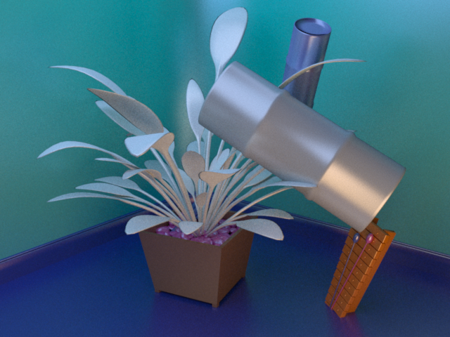
The main rendering uses path tracing light integration, 31 spectral planes, and enough lighting samples to "look good". This image was rendered by the Mitsuba renderer and converted to sRGB for visualization. The same is true of other renderings below.
This image illustrates a 'feature' of our object placement process, namely that it does not respect physical object boundaries, so that two objects may overlap in the 3D scene space in a manner that is not physically realistic. This can be seen here by the fact that one of the plant's leaves protrudes through the inserted barrel.
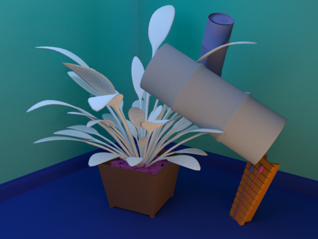
We repeat the "main" rendering for each scene, but this time we use only the diffuse reflectance component of each Ward material. Ignoring the randomness of the rendering process, this "matte" rendering should be equal to the main rendering minus the image component due to specular reflectances.
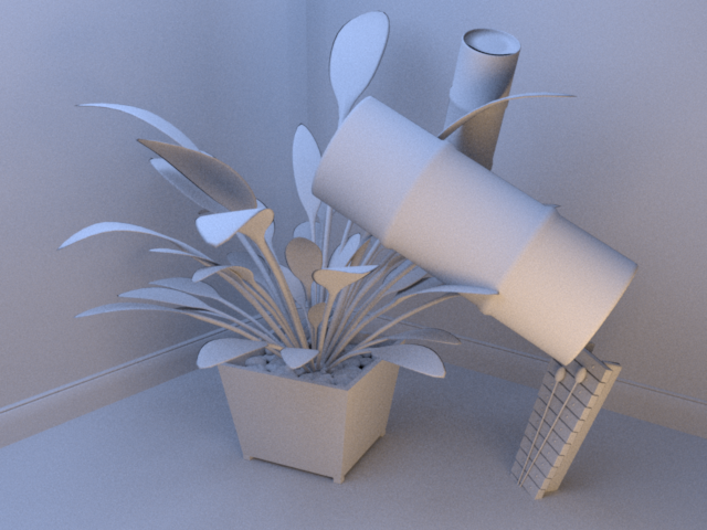
As a check on our intuition, we also render a "boring" variation on the main rendering. For this rendering we clobber all of the materials in the scene and assign a boring matte material with 50% reflectance at all wavelengths. This rendering should resemble the matte rendering in terms of lighting and geometry, but not in terms of interesting object reflectances.
For later analyses, we want to know which 3D-modeled object is located behind each pixel in the output image. We can determine this if we assign a unique, easy-to-identify reflectance to each object. So for the "mask" rendering we clobber all of the materials in the scene and assign a unique single-band reflectance to each object. We also clobber all of the lighting spectra and assign unit intensity at all wavelengths. This enables us to produce an object pixel mask, below.
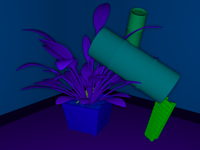
In this example, we have fewer than 31 objects in the scene. Since we're rendering with 31 spectral planes, we have enough single-band reflectances to go around. When we have more than 31 objects, we perform multiple mask renderings and stack them up during analysis.
After all renderings are done, we move on to image analysis.
We examine each pixel in the mask rendering to determine which object is behind it. Often this is obvious: we see reflected radiance in a single spectral band and we choose the object that had the corresponding single-band reflectance. At the edges between objects this is less obvious because multiple objects may have sent radiance into the same pixel.
We compute an object pixel mask that has at each pixel an id for the identified object, or else zero if we could not conclusively identify an object. We summarize the pixel mask with a "coverage" image. The coverage image is white where we managed to identify an object, and black where we could not.
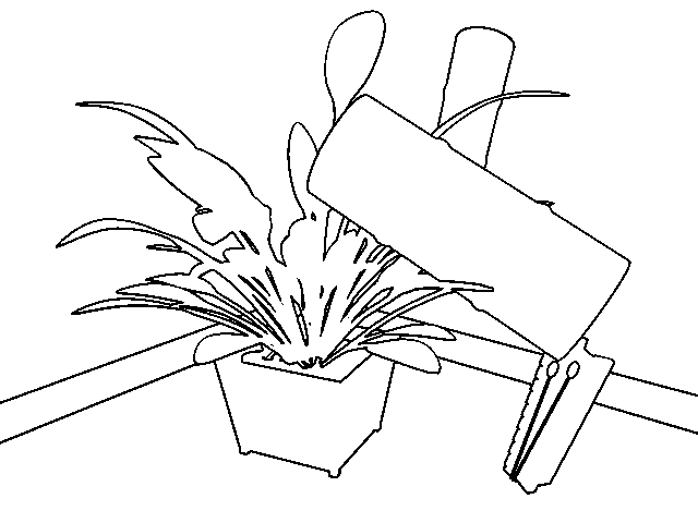
See function MakeRecipeObjectMasks.
Once we have the object pixel mask, we can form a "reflectance" image. This is a multi-spectral image that records the reflectance of the object behind each pixel in the matte rendering. We form the reflectance image by building a table of diffuse reflectances, one for each object in the scene, and then using the object pixel mask to index the table of reflectances.
The reflectance image contains a unit-less reflectance spectrum for each pixel. We imagine this as a flat "poster" model of the matte scene. For visualization, we can imagine rendering the poster model under spatially and spectrally uniform illumination. That is, we ignore the units and convert the reflectance image to sRGB as though it were a radiance image.
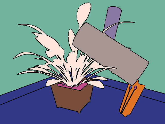
The reflectance image contains gaps everywhere the object pixel mask contains gaps. We fill in each gap pixel as the median of nearby non-gap pixels.
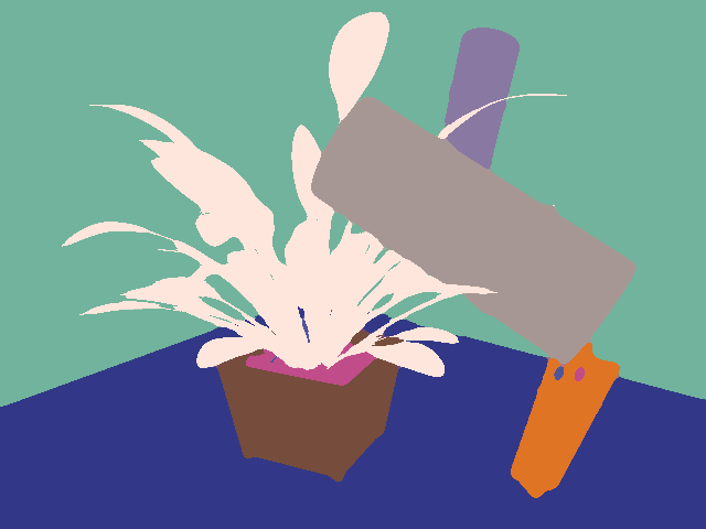
See function MakeRecipeIlluminationImage.
Once we have rendered radiance images and computed reflectance images, we can compute what we call 'illumination' images. These are of potential interest for those thinking about computational color constancy, where often we consider analyses based in the 2D image plane, and consider the possibility of separating images into reflectance and illumination planes (intrinsic images) that when multiplied together pixel by pixel produce the actual image. We do this analysis after stripping off the specular component as described above.
The basic illumination image is simply the rendered matte radiance image with the reflectance image "divided out". This uses the principle that the spectrum of radiance reflected from each object should be equal to the element-wise product of the object's reflectance spectrum and the spectrum of illumination arriving at the object, if we are thinking in the 2D image plane.
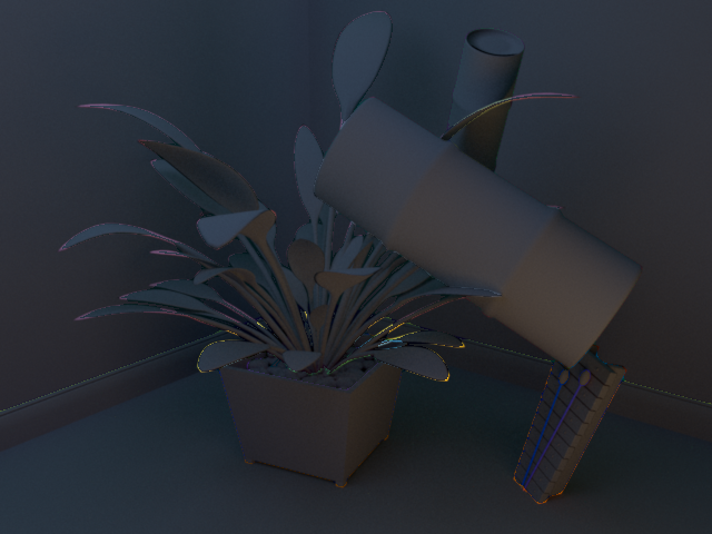
As with the reflectance image, we have to deal with the ambiguous pixels at the edges between objects. We use the same technique we used for reflectances, interpolation from nearby non-gap pixels, based on the object mask we generated above.
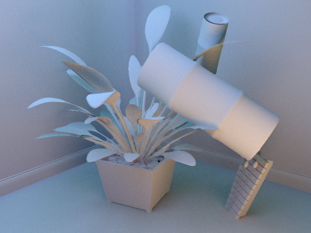
The image scaling of the two versions of the illumination image shown here differs because in each we normalize by the maximum value, and before the interpolation there are some extreme pixel values.
The illumination images reveal geometric variations across the surface of each object. We can ignore the geometric variations by computing the mean illumination across each object. We use the object pixel mask to identify which image regions to average across. Again, we interpolate the gap pixels.
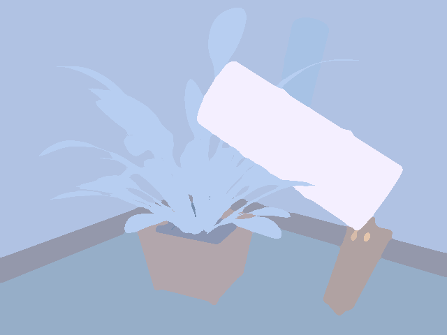
See function MakeRecipeIlluminationImage.
We are interested in photoreceptor responses to our computed images. We can model these responses using measured photoreceptor sensitivities.
We compute LMS images for our reflectance image, our illumination image, and our illumination-per-object image. We compute each of these as the image slice at each spectral plane, weighted by the sensitivity of the L, M, or S cone receptor at the corresponding wavelength.
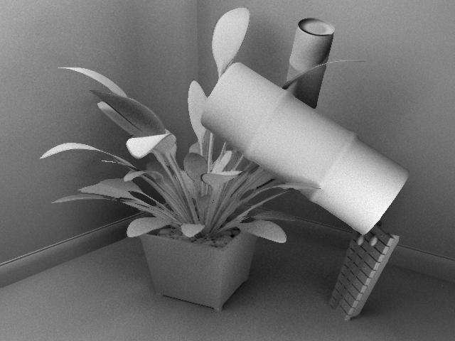
For visualization, we divide the computed LMS image by its max value. This allows the image to fill the entire [0 1] grayscale range. We use the same divisor for L, M, and S planes, so that their relative magnitudes are preserved in the visualization.
For example, here is the "L" component of the illumination image:
Here is the "M" component:
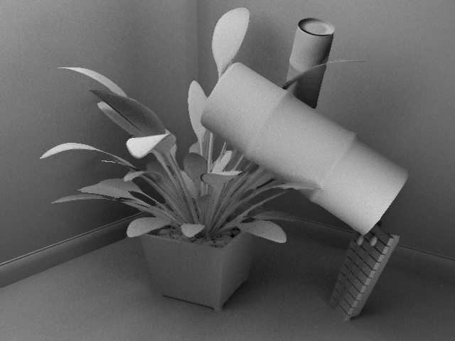
And here is the "S" component:
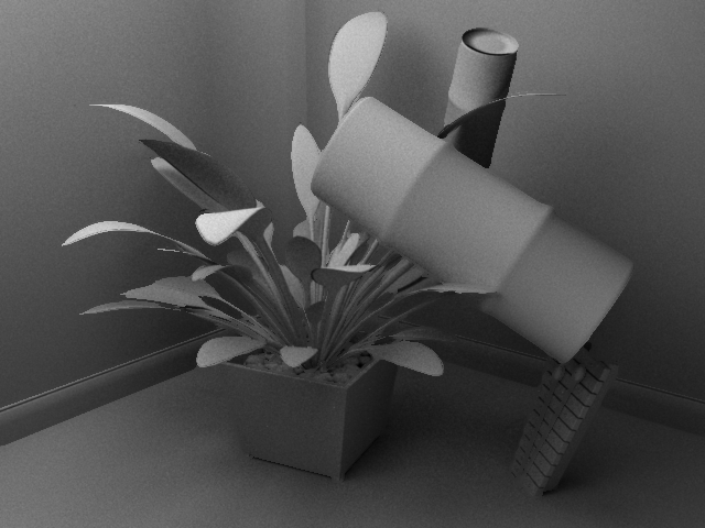
See function MakeRecipeLMSImages.
In addition to the LMS images for visualization, we produce a Matlab .mat file that has the actual image values for further analysis.
We are also interested in perceptual responses to our computed images. We can model some responses by converting our LMS images to DKL color space. This gives us an "l" image related to luminance, an "rg" image related to red-green color variation, and a "by" image related to blue-yellow color variation.
We compute DKL images for our reflectance image, our illumination image, and our illumination-per-object image.
For visualization we shift and scale each image separately to occupy most of the [0 1] grayscale range.
For example, here is the "l" component of the illumination image:
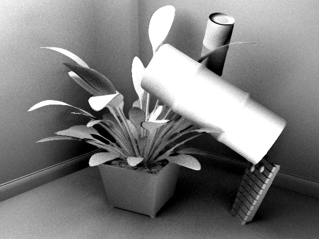
Here is the "rg" component:
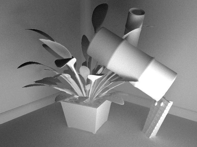
And here is the "by" component:
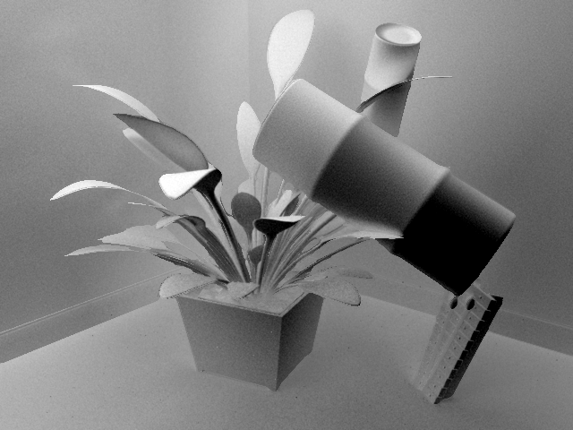
See functions MakeRecipeDKLImages and rtbDKLTutorial.
In addition to the DKL images for visualization, we produce a Matlab .mat file that has the actual image values for further analysis.
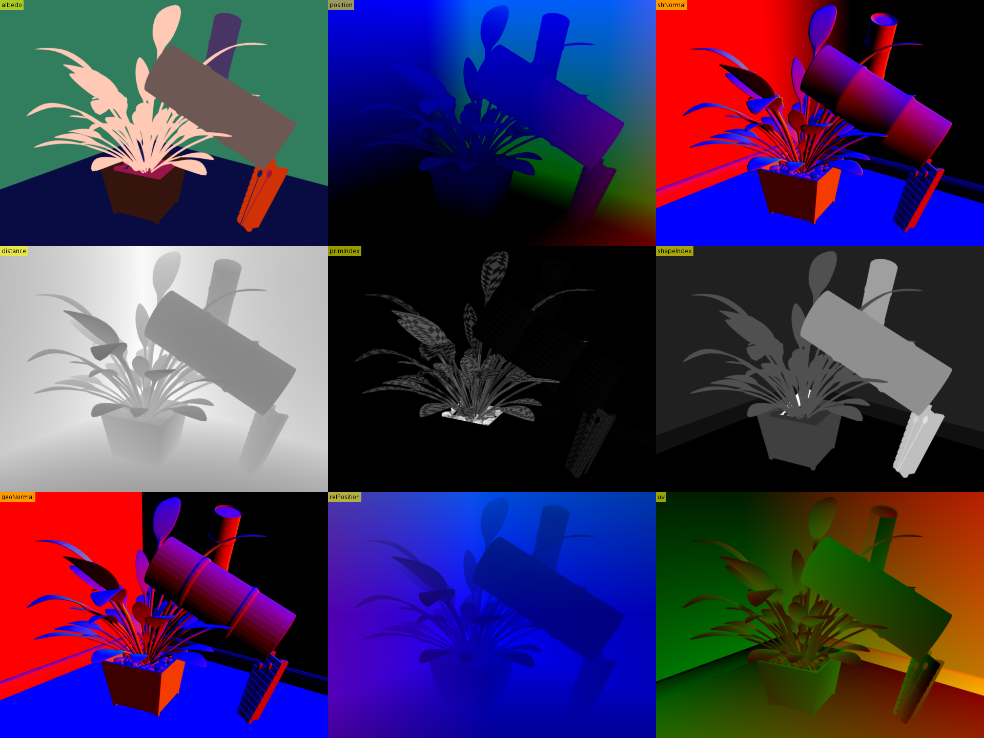
The Mitsuba renderer has a nice feature called the field integrator which allows us to extract extra data about a scene during rendering. We call these extra data "factoids".
The idea of a factoid is that for each output pixel, we get to look up a property of the scene object underneath that pixel. We can visualize each factoid as a false color image. For example, we can map XYZ scene coordinates to RGB image components.
Some of the factoid images resemble our object pixel masks and reflectance images.
We record all of the factoids that Mitsuba makes available. They are:
- albedo -- similar to our reflectance images
- distance -- distance from the camera to the surface under each pixel
- geoNormal -- the surface normal as used in geometric calculations
- shNormal -- the interpolated surface normal as used in shading calculations
- position -- the surface XYZ position in scene coordinates
- relPosition -- the surface XYZ position in camera coordinates
- primIndex -- identifies the low-level primitive shape that the surface belongs to
- shapeIndex -- similar to our object pixel mask
- uv -- the surface UV coordinates as used for texture mapping
Here is a montage with a false color image for each factoid (except albedo, which has some "true" color meaning). It's a large image, so you may wish to right-click and open it in a new window or tab.