Improving an Existing Partition
To use EnGPar's different algorithms, first the application must construct an N-graph from the user's data. To do this see Constructing the N-graph.
The general way to run EnGPar's load balancing procedures is in the following form:
  // C++
  agi::Balancer* balancer = engpar::callToBalancer(...)
  balancer->balance(tolerance)
If the goal is to balance out the vertices of the graph one can use the following function to construct a balancer that does so:
  agi::Balancer* engpar::makeVtxBalancer(agi::Ngraph* g,
                                         double stepFactor=0.1,
                                         int verbosity=0);
The first argument, g, is the graph. The second, stepFactor, controls how much
weight can be sent in a single iteration, and the final, verbosity, is the level
of output provided by EnGPar; the higher the value the more output. Note that
higher levels of verbosity can increase computation and communication costs.
To have more control over how EnGPar balances the graph a general balancer can be constructed with the following calls:
 engpar::Input* input = new engpar::Input(g);
 ai::Balancer balancer = makeBalancer(input,verbosity);
Various control mechanisms can be set in the input object in order to control
many aspects of how EnGPar works. See the header partition/engpar_input.h for more
information.
When using the FORTRAN interface, graph vertices can be balanced with the following call:
  // FORTRAN
  call cengpar_balanceVertices(graph, tol, stepfactor, verbosity);
Once the N-graph is balanced, the user data can be repartitioned using a partition map provided by the N-graph. To do this see Retrieving the Partition.
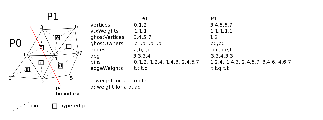
The figure above depicts a mixed mesh on two processes with a vertex-based
partition.
There are six mesh elements labelled a through f.
Five of the elements are triangles and one is a quadrilateral.
The eight mesh vertices are labelled 0 through 7.
Mesh edges are not labelled.
The mesh elements on each part are defined by the locally owned vertices, and
the elements they are adjacent to.
Vertices 0, 1, and 2 are owned by part 0, P0. The remaining vertices
are owned by part 1, P1.
Due to this assignment of vertices, elements c, b, and d span the part
boundary between P0 and P1 and exist on both parts.
The lists shown to the right of the figure define the information needed to create an Ngraph with hyperedges from this partitioned mesh. For each mesh vertex a graph vertex is created. Likewise, for each mesh element a hyperedge is created.
Locally owned mesh vertices, and their weights, are defined by the vertices
and vtxWeights lists.
For this example we assume that the graph vertices are uniformly weighted.
Next, the hyperedges, and their weights, are created via the edges and
edgeWeights lists.
In the figure a hyperedge is marked with a square.
Note that the elements spanning the part boundary (c,b, and d) exist in
the edges list of both P0 and P1.
The weights associated with each type of element are symbolically denoted as t
and q, respectively.
Additional information is needed to complete the definition of hyperedges from
mesh elements and the vertices on their closure.
First, the number of vertices on the closure of each element defines the degree
of the hyperedges; i.e., degree(triangle)=3 and degree(quad)=4.
Next, the list of vertices on the closure are listed in pins.
In the figure a pin is depicted as an hashed edge between a hyperedge and a vertex.
Finally, each non-local vertex that exists in the pins list is placed in the
ghostVertices list along with its corresponding remote process id in the
ghostOwners list.