Machine Learning - Classification Algorithms

Mateusz Dorobek - Data Science - Faculity of Mathematics and Information Science - Warsaw University of Technology

Project

Main goal of this project is to compare and find the best algorithm for binary classification problem.

• MATDOR contains predictions for belonging to class 1
• classifiers contains machine learning algorithms in R
• data_extraction contains data preparation script in Python

Data

Data used in this project comes from one of telecomunication company. They were anonimized, so data preparation couldn't base on expert experience. Unprocessed data can be found here. Preprocessing including standardization, encoding, factorization and other techniques was done with Python.

Assumption

I decided that if column has more than 99% of NaNs I'll remove it, so 23 columns went off. I've concatenated train and test set to perform the same data modyfications on both of them.

def load_data() -> pd.Series:
    csv_train = pd.read_csv('train.txt', sep=" ").assign(train = 1) 
    csv_test = pd.read_csv('testx.txt', sep=" ").assign(train = 0)
    csv = pd.concat([csv_train,csv_test])
    return csv

Very usefull was stat function which shows a lot of usefull statistics about column on screen

def stat(f):
    nans = nans_ctr()
    unique = unique_ctr()
    val_type = val_types()
    print(f"min: {csv[f].min()}")
    print(f"max: {csv[f].max()}")
    print(f"nans: {nans[f]}")
    print(f"unique: {unique[f]}")
    print(f"val_type: {val_type[f]}")
    print(f"vals per class: {round((len(csv)-nans[f])/unique[f],2)}")

Data Processing

Data that I had pleasure to work with had almost 30% of NaNs, so I've to fill them up. My idea is basicly filling next row NaNs with value from previous no-empty value in that column. This method is in a lot of cases similar to median and mean, but has two main advantages over them.

• Is immune to oultiers compared to mean.
• Has higher variance than median, not causing peak in distributon.

...
csv[f] = csv[f].fillna(method='ffill')
csv[f] = csv[f].fillna(method='bfill')

I've used factorize on string data to convert them to separable numeric classes

def factorize(data) -> pd.Series():
    series = data.copy()
    labels, _ = pd.factorize(series)
    series = labels[:len(series)]
    return series

I've used threshold_factorization on data, where was a lot of text values (more than 10) not connected eachother, so I've decided to calculate quantity and split them in several groups based on their number.

def threshold_factorization(data, *t_list) -> pd.Series():
   letter_counts = Counter(data)
      df = pd.DataFrame.from_dict(letter_counts, orient='index')
      df = df.sort_values(by=0, ascending=False)
      t_list = (df.values[0].item()+1,) + t_list + (0,)
      out = data.copy()
      for i in tqdm(range(1,len(t_list)),desc="Progress",leave=False):
          idx = df[(df>t_list[i]).values & (df<=t_list[i-1]).values].index
          for j in tqdm(idx,leave=False):
              out.loc[out == j] = i
      return out

Example of such distribution

...
plot(csv[f],sort=True,log=True,fontsize=14,small=True)
csv[f] = threshold_factorization(csv[f],900,100,10,1)
plot(csv[f],sort=True,log=True,fontsize=14,small=True)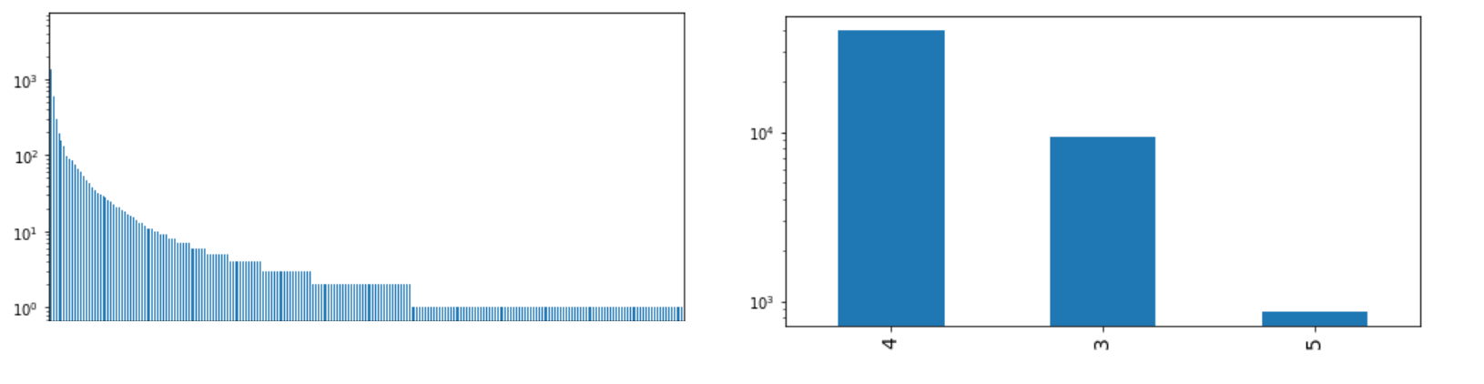

I've used cast to limit range of columns with long distribution tail, casting large values to some lower.

def cast(data, lower_t, upper_t) -> pd.Series():
    data = data.sort_values()
    data[data<lower_t] = lower_t
    data[data>upper_t] = upper_t
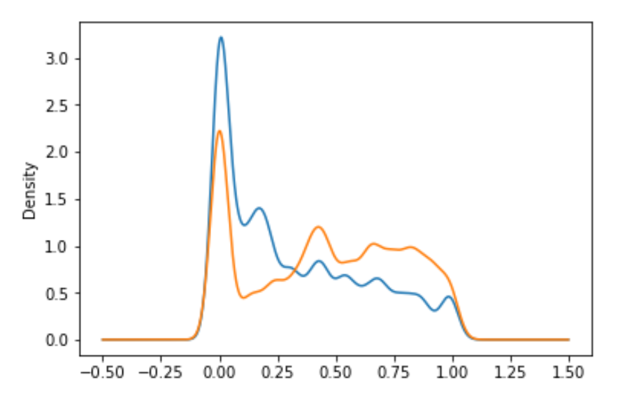
    return data

Example of such distribution

...
csv[f].plot.kde()
csv[f] = cast(csv[f],-100,csv[f].quantile(0.98))
csv[f].plot.kde()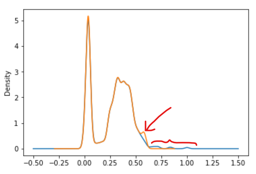

I've used standarization, by reducing range to <0,1>

def standarize(df) ->pd.Series():
    return round((df-df.min())/(df.max()-df.min()),4)

I've used transformation that tilts distribution in cases, where most of examples had value near one of sides, and differences beetween them will very small. It may cause model not to learn difference between them.

...
ax = csv[f].plot.kde()
csv[f] = csv[f].apply(lambda x: np.power(x,1/2))
csv[f] = standarize(csv[f])
csv[f].plot.kde()

In this example differences in lower part are more important (due to a lot of examples in that region), but difference between them is very small, so I've spreaded tehm and moved a little bit to right side using lambda.

One thing that I've done several times is encoding. I've use One Hot Encoding in smaller number of classes and Binary Encoding, when I had more than 3 classes, to reduce number of created columns.

def one_hot_encoding(f):
    global csv
    ohe = ce.OneHotEncoder(cols = [f], handle_unknown='ignore', use_cat_names=True)
    csv[f] = csv[f].fillna(-1)
    new_features = ohe.fit_transform(csv[f].to_frame())
    csv = csv.drop([f],axis=1)
    csv = pd.concat([csv,new_features],axis=1)
    
def binary_encoding(f):
    global csv
    ohe = ce.BinaryEncoder(cols = [f], handle_unknown='ignore',drop_invariant=True)
    csv[f] = csv[f].fillna(-1)
    new_features = ohe.fit_transform(csv[f].to_frame())
    csv = csv.drop([f],axis=1)
    csv = pd.concat([csv,new_features],axis=1)  

Algorithms

To perform classification and choose the best algorithm I've used R. Whole script you can find at my GitHub at this link I've used 20% of training data as validation set.

Extremely Randomized Trees

extraTrees(x = train_no_class, y = train$class,  ntree=500, numThreads = 8)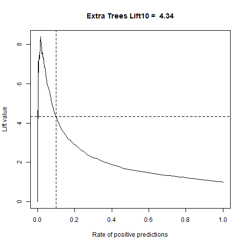

Random Forest

randomForest(class ~ ., data = train)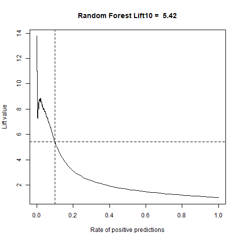

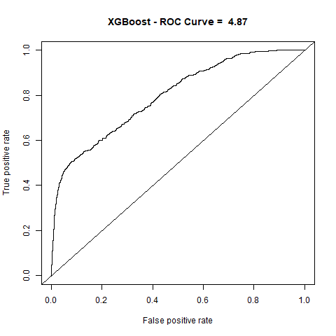
XGBoost

xgboost(
  data = data.matrix(train_no_class),
  label = as.numeric(as.vector(train$class)),
  nrounds = 2000,
  max.depth = 4,
  eta = 0.07,
  nthreads = 8,
  objective = "binary:logistic"
)

Generalized Boosted Regression Modeling

gbm(class ~ ., data = train, distribution = "gaussian")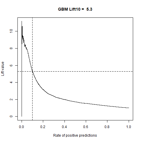

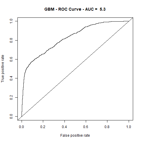
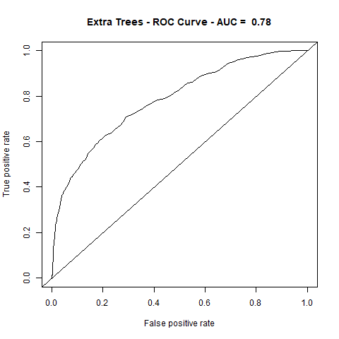
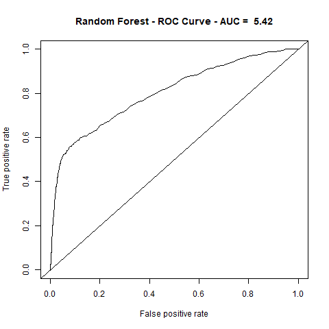
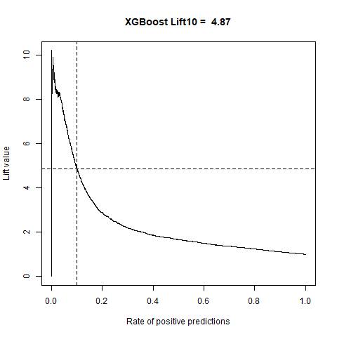
Summarise

For final algoritm I've choosen GBM, because it has the highest AUC measure, and despite its Lift10 measure is slightly lower than Random Forest I think that GMB Lift Curve is more stable, and for most of the time is higher than Random Forest List Curve, as you can see in last - zoomed image.

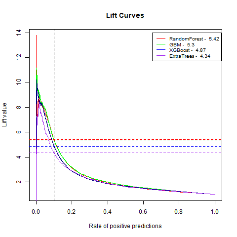
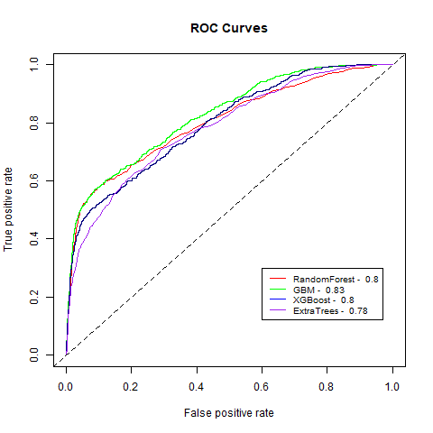
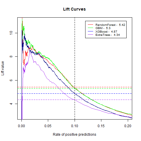
Name	Lift10	AUC
ExtraTrees	4.34	78%
RandomForest	5.42	80%
XGBoost	4.87	80%
GBM	5.30	83%