piscine_python_ml

Bootcamp Python

# For bootcamp python
export PYTHONPATH=/home/rcutte/Desktop/piscine_python_ml/bootcamp_python

Types

More infos

• 🐍 Python - Built-in Types
  • https://docs.python.org/3/library/stdtypes.html#truth-value-testing
  • https://docs.python.org/3/library/stdtypes.html#numeric-types-int-float-complex
  • https://docs.python.org/3/library/stdtypes.html#numeric-types-int-float-complex
  • https://docs.python.org/3/library/stdtypes.html#sequence-types-list-tuple-range
  • https://docs.python.org/3/library/stdtypes.html#text-sequence-type-str
  • https://docs.python.org/3/library/stdtypes.html#set-types-set-frozenset
  • https://docs.python.org/3/library/stdtypes.html#mapping-types-dict

classDiagram
    class object {
        <<built-in>>
    }
    class int {
        <<built-in>>
    }
    class float {
        <<built-in>>
    }
    class str {
        <<built-in>>
    }
    class list {
        <<built-in>>
    }
    class dict {
        <<built-in>>
    }
    class tuple {
        <<built-in>>
    }
    class set {
        <<built-in>>
    }

    object <|-- int
    object <|-- float
    object <|-- complex
    object <|-- str
    object <|-- list
    object <|-- dict
    object <|-- tuple
    object <|-- set

    note for object "Base class of all Python objects"
    note for int "Whole numbers (e.g., 1, 2, 3)"
    note for float "Decimal numbers (e.g., 3.14, -0.5)"
    note for complex "Complex numbers (e.g., 3+4j)"
    note for str "Text strings (e.g., 'hello', \'\'world\'\')"
    note for list "Ordered collections (e.g., [1, 2, 3])"
    note for dict "Key-value mappings (e.g., {'a': 1})"
    note for tuple "Immutable ordered collections (e.g., (1, 2, 3))"
    note for set "Unordered unique elements (e.g., {1, 2, 3})"

Loading

Dict

More infos

• 🐍 Python - Dictionaries

flowchart LR
    classDef basic fill:#90EE90,stroke:#006400,color:#000000
    classDef modify fill:#FFB6C1,stroke:#8B0000,color:#000000
    classDef query fill:#ADD8E6,stroke:#000080,color:#000000

    Start["Dictionary Operations"] --> Basic["Basic Operations"]
    Start --> Modify["Modification"]
    Start --> Query["Query Operations"]

    subgraph "Basic Operations"
        Basic --> Create["Creation
        d = {}"]
        Basic --> Access["Access
        d[key]"]
        Basic --> Check["Check Existence
        key in d"]
    end

    subgraph "Modification"
        Modify --> Add["Add/Update
        d[key] = value"]
        Modify --> Delete["Delete
        del d[key]<br>d.pop(key, return_value)"]
        Modify --> Clear["Clear All
        d.clear()"]
    end

    subgraph "Query Operations"
        Query --> Keys["Get Keys
        d.keys()"]
        Query --> Values["Get Values
        d.values()"]
        Query --> Items["Get Items
        d.items()"]
    end

    class Basic,Create,Access,Check basic
    class Modify,Add,Delete,Pop,Clear modify
    class Query,Keys,Values,Items query

Loading

Formating

More infos

• 🐍 Python - Format Specification Mini-Language

flowchart LR
    classDef basic fill:#90EE90,stroke:#006400,color:#000000
    classDef advanced fill:#FFB6C1,stroke:#8B0000,color:#000000
    classDef output fill:#ADD8E6,stroke:#000080,color:#000000

    Start["String Formatting"] --> Basic["Basic Methods"]
    Start --> Advanced["Advanced Methods<br><br>[[fill]align][sign][#][0][width][grouping_option][.precision][type]"]

    subgraph "Basic Methods"
        Basic --> F["f-strings
        name = 'John'
        f'Hello, {name}!'"]
        Basic --> Format["str.format()
        'Hello, {}!'.format(name)"]
        Basic --> Percent["% Operator
        'Hello, %s!' % name"]
    end

    subgraph "Advanced Methods"
        Advanced --> Align["Alignment
        '{:-^10}'.format(name)"]
        Advanced --> Fill["Fill Character
        '{:_>10}'.format(name)"]
        Advanced --> Width["Width Specifier
        '{:10}'.format(name)"]
        Advanced --> Precision["Precision
        '{:.2f}'.format(3.14159)"]
    end

    F --> Output1["Output:
    Hello, John!"]
    Format --> Output2["Output:
    Hello, John!"]
    Percent --> Output3["Output:
    Hello, John!"]
    Fill --> Output4["Output:<br>______John"]
    Align --> Output5["Output:<br>---John---"]
    Width --> Output6["Output:
    John"]
    Precision --> Output7["Output:
    3.14"]

    class Basic,Format,F,Percent basic
    class Advanced,Align,Width,Precision,Fill advanced
    class Output1,Output2,Output3,Output4,Output5,Output6,Output7 output

Loading

Vectors

📹 Youtube - Vectors - Essence of linear algebra 🐍 Python - datamodel - numeric types

Builtins functions

• 🐍 Python - Builtin Functions
  • https://docs.python.org/3.9/library/functions.html#vars
  • https://docs.python.org/3.9/library/functions.html#dir

Decorators

Decorators

• 🐍 Python - Decorators

sequenceDiagram
    participant C as Client Code
    participant D as Decorator (@my_decorator)
    participant W as Wrapper Function
    participant O as Original Function

    Note over C,O: Normal Execution Flow
    C->>+D: Call decorated function
    D->>+W: Execute wrapper
    Note over W: Before function code runs
    W->>+O: Call original function
    O-->>-W: Return from original
    Note over W: After function code runs
    W-->>-D: Return to decorator
    D-->>-C: Final return to client

    Note over C,O: Equivalent Manual Decoration
    C->>D: my_decorator(original_function)
    D-->>C: Returns decorated function

Loading

Best Practices

1. Always use functools.wraps to preserve the original function's metadata:

from functools import wraps

def my_decorator(func):
    @wraps(func)  # Preserves function name, docstring, etc.
    def wrapper(*args, **kwargs):
        return func(*args, **kwargs)
    return wrapper

2. Handle arguments properly using *args and **kwargs:

def flexible_decorator(func):
    def wrapper(*args, **kwargs):
        print(f"Received args: {args}, kwargs: {kwargs}")
        return func(*args, **kwargs)
    return wrapper

Context Managers

More infos

• 🐍 Python - Context Managers

sequenceDiagram
    participant C as Client Code
    participant W as With Statement
    participant CM as Context Manager

    Note over C,CM: Normal Execution
    C->>W: Enter with block
    W->>CM: __enter__()
    CM-->>W: Return value
    W->>C: Assign to 'as' variable
    Note over C: Execute block content
    C->>W: Block complete
    W->>CM: __exit__(None, None, None)

    Note over C,CM: Exception Case
    C->>W: Enter with block
    W->>CM: __enter__()
    CM-->>W: Return value
    W->>C: Assign to 'as' variable
    Note over C: Execute block content
    C->>W: Raise Exception
    W->>CM: __exit__(exc_type, exc_val, traceback)
    alt __exit__ returns True
        CM-->>W: Suppress exception
    else __exit__ returns False
        CM-->>W: Propagate exception
    end

Loading

Package

🐍 Python - Creating a packgage - https://packaging.python.org/en/latest/tutorials/packaging-projects/#packaging-python-projects - https://docs.python.org/3/tutorial/modules.html#packages - Setuptools - Config

# Setup the env
python3 -m venv .venv
source .venv/bin/activate

pip install setuptools wheel twine

# Setup your package

# After setting up the package - update build
python3 -m pip install --upgrade build

# Build the package
python3 -m build

📜 Choose a license

Numpy

• https://numpy.org/doc/2.2/
• https://numpy.org/doc/2.2/user/absolute_beginners.html
• https://numpy.org/doc/2.2/reference/index.html
• https://numpy.org/doc/2.2/user/basics.broadcasting.html#basics-broadcasting

Matplotlib

https://matplotlib.org/stable/contents.html https://matplotlib.org/stable/users/explain/quick_start.html

Plot Setup

https://matplotlib.org/stable/api/_as_gen/matplotlib.pyplot.scatter.html#matplotlib.pyplot.scatter

Plot Colors and markers

https://matplotlib.org/stable/api/markers_api.html#module-matplotlib.markers https://matplotlib.org/stable/users/explain/colors/colormaps.html#sphx-glr-users-explain-colors-colormaps-py

Pandas

• https://pandas.pydata.org/docs/getting_started/index.html#intro-to-pandas
• https://pandas.pydata.org/docs/user_guide/10min.html#min
• https://pandas.pydata.org/docs/
• https://pandas.pydata.org/docs/user_guide/index.html

Bootcamp ML

# For importing the bootcamp_ml and bootcamp_python modules
export PYTHONPATH=/home/rcutte/Desktop/piscine_python_ml

Machine Learning

• coursera - Machine Learning
• youtube - Machine Learning

mindmap
    root((Machine Learning))
        (Supervised Learning)
            (Classification)
                (Binary/Multi-class)
                (Image Recognition)
                (Sentiment Analysis)
            (Regression)
                (Numerical Prediction)
                (Continuous Values)
        (Unsupervised Learning)
            (Clustering)
                (Group Similar Data)
                (Customer Segmentation)
            (Dimensionality Reduction)
                (Feature Selection)
                (Data Visualization)
            (Anomaly Detection)
                (Outlier Identification)
                (Fraud Detection)
        (Reinforcement Learning)
            (Value-Based Methods)
                (Q-learning)
                (Deep Q-Networks)
            (Policy-Based Methods)
                (REINFORCE)
                (PPO)
            (Actor-Critic Methods)
                (A2C)
                (SAC)

Loading

Types

There are 4 types of machine learning:

• Supervised Learning
• Unsupervised Learning
• Recommender Systems
• Reinforcement Learning

Supervised Learning

"Learn from right answers"

Helps to predict the output when given an input.

Input (X)	Output (Y)	Application Examples
House Features	Price	Real Estate Pricing
Email Content	Spam/Not Spam	Email Filtering
Medical Images	Disease/No Disease	Medical Diagnosis
Audio Files	Text Transcript	Speech Recognition
Historical Prices	Future Prices	Stock Prediction
Image of a product	Defects	Quality Control

Regression

• Predict continuous valued output
  • Predict a number: infinite number of values
• E.g., predict house price

Linear Regression

• Simplest form of regression
• Assumes linear relationship between input and output
• E.g., predict house price based on size

Univariate Linear Regression

One feature (input variable) and one target variable (output variable).

• $f_{w,b}(x) = w x + b$
  • $w$ = slope
  • $b$ = y-intercept

Cost Function: Mean Squared Error (MSE)

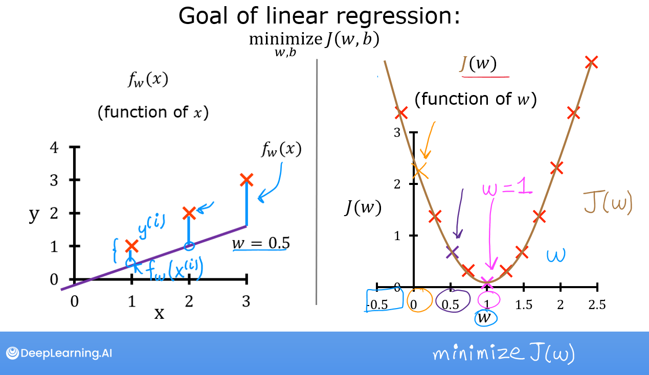
• Measures the average of the squares of the errors or deviations

  • E.g., difference between predicted and actual value $$ \begin{align*} \text{Error} & = \text{Estimate} - \text{Actual value} = \hat{y} - y \ \text{Total Errors} & = \sum_{i=1}^{m} (\hat{y}^{(i)} - y^{(i)})^2 \ \text{Mean Squared Error} & = \frac{1}{m} \sum_{i=1}^{m} (\hat{y}^{(i)} - y^{(i)})^2 \ \text{Cost Function} & = \frac{1}{2m} \sum_{i=1}^{m} (\hat{y}^{(i)} - y^{(i)})^2 \ & \text{where } \frac{1}{2} \text{ is used to simplify the derivative} \ & \hat{y}^{(i)} = f_{w,b}(x^{(i)}) = w x^{(i)} + b \ J_{w,b} & = \frac{1}{2m} \sum_{i=1}^{m} (f_{w,b}(x^{(i)}) - y^{(i)})^2 \ \end{align*} \ $$

• Goal: minimize the cost function

  • Find the best values for $w$ and $b$
    • Simplified : $J_{w}$ = cost function with respect to $w$
  • E.g., find the best fit line

• Contour plot: visualize the cost function
  • 2D plot: $w$ and $b$ on the x and y axes
  • Color: cost function value
  • Helps find the minimum of the cost function

Gradient Descent

• Optimization algorithm used to minimize the cost function

• Update parameters $w$ and $b$ to reduce the cost function

• Repeat until convergence

  • E.g., find the minimum of the cost function

• Learning rate ($\alpha$) = step size

  • always positive
  • small: slow convergence
  • large: may overshoot the minimum

• Partion derivative ($\partial$) = slope of the cost function

• Update rule:

  • $w :=\greenD{w} - \blueD{\alpha} \goldD{\frac{\partial}{\partial w} J_{w,b}} = \greenD{w} - \blueD{\alpha} \goldD{ \frac{1}{m} \sum_{i=1}^{m} (f_{w,b}(x^{(i)}) - y^{(i)}) x^{(i)}}$
    • $\goldD{\text{Derivative (simplified)}}$
    • $\blueD{\text{Learning rate / Step size}}$
    • $\greenD{Parameter}$
  • $b := b - \alpha \frac{\partial}{\partial b} J_{w,b} = b - \alpha \frac{1}{m} \sum_{i=1}^{m} (f_{w,b}(x^{(i)}) - y^{(i)})$

• Calculate simultaneously and Repeat until convergence:

  • $tmp_w := w - \alpha \frac{\partial}{\partial w} J_{w,b}$
  • $tmp_b := b - \alpha \frac{\partial}{\partial b} J_{w,b}$
  • $w := tmp_w$
  • $b := tmp_b$

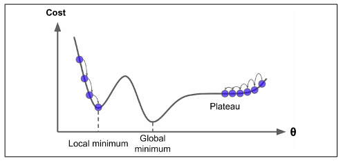
• Local minimum: point where the cost function is lower than its value at any neighboring points

  • Gradient descent may converge to a local minimum
  • As we get closer to the minimum, the derivative approaches zero
    • At the minimum, the derivative is zero (flat slope)
  • With squared error cost function, the cost function is convex
    • Only one minimum
  • Convex function: any local minimum is a global minimum

• Global minimum: point where the cost function is lower than its value at any other point

• Batch gradient descent: use all training examples in each iteration

  • Computationally expensive for large datasets

• Multivariate Linear Gradient:
  • $\nabla_{\vec{w}} J_{\vec{w},b} = \frac{1}{m} \sum_{i=1}^{m} (f_{\vec{w},b}(\vec{x}^{(i)}) - y^{(i)}) \vec{x}^{(i)}$
  • $\nabla(J) = \frac{1}{m} X'^T (X' \vec{w} - \vec{y})$
    • $X'$ = input matrix with an additional column of ones for the bias
      • $X' = \begin{bmatrix} 1 & x_1^{(1)} & x_2^{(1)} & \ldots & x_n^{(1)} \ 1 & x_1^{(2)} & x_2^{(2)} & \ldots & x_n^{(2)} \ \vdots & \vdots & \vdots & \ddots & \vdots \ 1 & x_1^{(m)} & x_2^{(m)} & \ldots & x_n^{(m)} \end{bmatrix}$
    • $\vec{w}$ = weight vector = $[b, w_1, w_2, \ldots, w_n]$
    • $\vec{y}$ = target vector
    • $X'^T$ = transpose of $X'$
  • $\nabla(J)$ Gradient vector

Multiple Linear Regression

Not multivariate linear regression (multiple target variables) but multiple features (input variables).

$$ \begin{aligned} \begin{bmatrix} x_{\goldD{1}}^{\blueD{(1)}} & x_{\goldD{2}}^{\blueD{(1)}} & \ldots & x_{\goldD{n}}^{\blueD{(1)}} \\ x_{\goldD{1}}^{\blueD{(2)}} & x_{\goldD{2}}^{\blueD{(2)}} & \ldots & x_{\goldD{n}}^{\blueD{(2)}} \\ \vdots & \vdots & \ddots & \vdots \\ x_{\goldD{1}}^{\blueD{(m)}} & x_{\goldD{2}}^{\blueD{(m)}} & \ldots & x_{\goldD{n}}^{\blueD{(m)}} \\ \end{bmatrix} \cdot \begin{bmatrix} w_{\goldD{1}} \\ w_{\goldD{2}} \\ \vdots \\ w_{\goldD{n}} \\ \end{bmatrix} + b \\ &\text{\goldD{n} = number of features} \\ &\text{\blueD{m} = number of training examples} \end{aligned} $$

• $f_{w,b}(x) = w_1 x_1 + w_2 x_2 + \ldots + w_n x_n + b = f_{\vec{w},b}(\vec{x}) = \vec{w} \cdot \vec{x} + b$
  • $\vec{w} = [w_1, w_2, \ldots, w_n]$
  • $\vec{x}^{\blueD{(i)}} = [x_1, x_2, \ldots, x_n]$ = feature vector of the $\blueD{i^{th}}$ training example
  • $b$ is a number also known as the bias
  • $x_{\goldD{j}}^{\blueD{(i)}}$ = value of feature $\goldD{j}$ in the $\blueD{i^{th}}$ training example

Feature scaling:

• Helps gradient descent converge more quickly
  • E.g., scale features to have a similar range of values
• Aim for a mean of zero and a range of -1 to 1
  • $-1 \leq x_{\goldD{j}} \leq 1$ for each feature $\goldD{j}$
• Mean normalization:
  • subtract the mean and divide by the range
  • $x_{\goldD{j}} = \frac{x_{\goldD{j}} - \mu_{\goldD{j}}}{\sigma_{\goldD{j}}}$
    • $\mu_{\goldD{j}}$ = mean of feature $\goldD{j}$
      • $\mu_{\goldD{j}} = \frac{1}{m} \sum_{i=1}^{m} x_{\goldD{j}}^{\blueD{(i)}}$
    • $\sigma_{\goldD{j}}$ = range of feature $\goldD{j}$
      • $\sigma_{\goldD{j}} = \max(x_{\goldD{j}}) - \min(x_{\goldD{j}})$
• Z_score normalization:
  • subtract the mean and divide by the standard deviation
  • $x_{\goldD{j}} = \frac{x_{\goldD{j}} - \mu_{\goldD{j}}}{\sigma_{\goldD{j}}}$
    • $\mu_{\goldD{j}}$ = mean of feature $\goldD{j}$
      • $\mu_{\goldD{j}} = \frac{1}{m} \sum_{i=1}^{m} x_{\goldD{j}}^{\blueD{(i)}}$
    • $\sigma_{\goldD{j}}$ = standard deviation of feature $\goldD{j}$
      • $\sigma_{\goldD{j}} = \sqrt{\frac{1}{m} \sum_{i=1}^{m} (x_{\goldD{j}}^{\blueD{(i)}} - \mu_{\goldD{j}})^2}$

Classification

• Predict discrete valued output
  • Predict categories or labels: small number of discrete values
• E.g., predict spam or not spam

Unsupervised Learning

"Learn from unlabeled data"

Helps to find patterns in data. - Only input data (no output data)

Input (X)	Application Examples
Customer Data	Customer Segmentation
News Articles	Topic Modeling
Audio Files	Music Genre Classification
Image Data	Image Clustering
Sensor Data	Anomaly Detection
DNA Sequences	Gene Expression Analysis

Clustering

• Group similar data points together
• E.g., customer segmentation

Anomaly Detection

• Identify unusual data points
• E.g., fraud detection

Dimensionality Reduction

• Compress data using fewer numbers, while preserving the most important information
• E.g., data visualization

Notation

• $m$ = number of training examples
• $x$ = input variable/features
• $y$ = output variable/target
• $(x, y)$ = one training example
• $(x^{(i)}, y^{(i)})$ = $i^{th}$ training example
  • $i^{th}$ = index into training set ($i$ is an index, not an exponent) $\neq$
• $X$ = input matrix
• $Y$ = output matrix
• $f$ = target function / model
• $w, b$ = $\theta$ = parameters / coefficients / weights
• $\hat{y}$ = predicted output / estimate for $y$
• $h$ = hypothesis function
  • $h_{w,b}(x) = w x + b$
  • $h_{\theta}(x) = \theta x$
• $J$ = cost function
• $\alpha$ = learning rate
• $\partial$ = partial derivative

Math

• Math - symbols

---
title: Mathematical Concepts
config:
    theme: default
---
mindmap
    root((Mathematical<br/>Concepts))
        Linear Algebra
            Vectors
            Matrices
            Transformations
            Eigenvalues
            Determinants
        Descriptive Statistics
            Central Tendency
                Mean
                Median
                Mode
            Dispersion
                Variance
                Standard Deviation
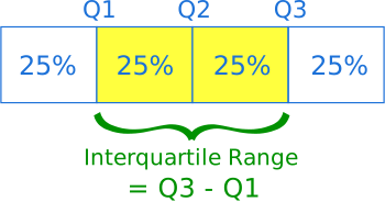
                Quartiles
            Shape Description
                Skewness
                Kurtosis

Loading

Visualization

• 3D Geogebra

Statistics

Central Tendency

• Mean: https://www.mathsisfun.com/mean.html
• Median: https://www.mathsisfun.com/median.html

K-Means

https://neptune.ai/blog/k-means-clustering https://www.geeksforgeeks.org/k-means-clustering-introduction/

Dispersion

• Quartiles: https://www.mathsisfun.com/data/quartiles.html

• Standard Deviation and Variance: https://www.mathsisfun.com/data/standard-deviation.html

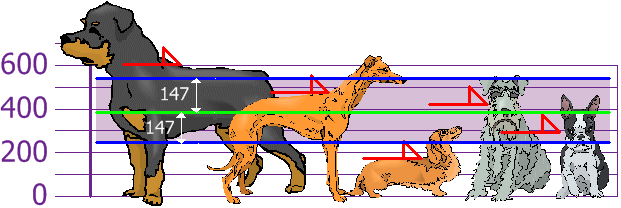
  • Variance: average of the squared differences from the Mean ($\bar{x}$) $$ \begin{aligned} \text{Variance} = \frac{\sum_{i=1}^{n} (x_i - \bar{x})^2}{n} \end{aligned} $$

  • Standard Deviation: square root of the Variance

    • Measures the amount of variation or dispersion of a set of values $$ \begin{aligned} \text{Standard Deviation} = \sqrt{\text{Variance}} \end{aligned} $$

Linear Algebra

L1 and L2

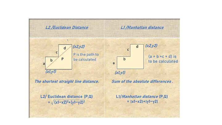
• L1 - Manhattan Distance
  • Also: Taxicab Distance
  • Measures the distance between two points as if you were traveling along a city grid and can only move along the streets (no diagonals).
  • May be preferred when dimensions are not of the same scale.
• L2 - Euclidean Distance
  • Measures the distance between two points as if you could travel through the air (no obstacles).
  • More sensitive to differences in magnitude between dimensions.

Difference betwenn L1 and L2

Vectors

📹 Youtube - Vectors - Essence of linear algebra

Operations

• Dot product:
  • $a \cdot b = a_1 b_1 + a_2 b_2 + \ldots + a_n b_n$

Matrices

📹 Youtube - Matrices - Essence of linear algebra

Operations

• Addition and Subtraction: https://www.khanacademy.org/math/algebra-home/alg-matrices/alg-adding-and-subtracting-matrices/a/adding-and-subtracting-matrices
• Multiplication and division:
  • scalar: https://www.khanacademy.org/math/algebra-home/alg-matrices/alg-multiplying-matrices-by-scalars/a/multiplying-matrices-by-scalars
    • Case: $$ \begin{aligned} \greenD 2\bold A&=\greenD{2}\cdot{\left[\begin{array}{c} 10 &6 \\ 4& 3 \end{array}\right]} \\ &={\left[\begin{array}{c} \greenD2 \cdot10 &\greenD2\cdot 6 \\ \greenD2\cdot 4& \greenD2\cdot3 \end{array}\right]} \\ &=\left[\begin{array}{c} 20 &12 \\ 8& 6 \end{array}\right] \end{aligned} $$
  • matrix: https://www.khanacademy.org/math/algebra-home/alg-matrices/alg-matrix-multiplication/v/matrix-multiplication-intro

    • Rules:

      • The number of columns in the first matrix must be equal to the number of rows in the second matrix.
      • The resulting matrix will have the same number of rows as the first matrix and the same number of columns as the second matrix. $$ \begin{aligned} \bold{A} \cdot \bold{B} &= \bold{AB}\ \blueD{m \times \goldD{n}} \cdot \goldD{n \times \blueD{p}} &= \blueD{m \times p}\ &\text{Equal: }\goldD{n}\ &\text{Dimension of AB: } \blueD{m, p} \end{aligned} $$

    • Structure: $$ \begin{array}{rccc} &\goldD{\vec{c_1}}&\goldD{\vec{c_2}}&\goldD{\vec{c_3}}\ &\goldD\downarrow&\goldD\downarrow&\goldD\downarrow \\ \begin{array}{c}\blueD{\vec{r_1}\rightarrow} \\blueD{\vec{r_2}\rightarrow} \\blueD{\vec{r_3}\rightarrow}\end{array} &\left[\begin{array}{c}1\6\2\end{array}\right. &\begin{array}{c}3\3\1\end{array} &\left.\begin{array}{c}5\7\4\end{array}\right] \end{array} $$

    • Case: $\greenD{c_{1,2}}$ is the dot product of $\blueD{\vec{a_1}}$ and $\goldD{\vec{b_2}}$ $$ \begin{array}{ccccccccc} &&&&\goldD{\vec{b_1}}&\goldD{\vec{b_2}} \ &&&&\goldD\downarrow&\goldD\downarrow \\ \begin{array}{c}\blueD{\vec{a_1}\rightarrow} \\blueD{\vec{a_2}\rightarrow}\end{array} &\left[\begin{array}{c}1\2\end{array}\right. &\left.\begin{array}{c}7\4\end{array}\right] &\cdot &\left[\begin{array}{c}3\5\end{array}\right. &\left.\begin{array}{c}3\2\end{array}\right] &= &\left[\begin{array}{c}\blueD{\vec{a_1}}\cdot\goldD{\vec{b_1}}\\blueD{\vec{a_2}}\cdot\goldD{\vec{b_1}}\end{array}\right. &\left.\begin{array}{c}\blueD{\vec{a_1}}\cdot\goldD{\vec{b_2}}\\blueD{\vec{a_2}}\cdot\goldD{\vec{b_2}}\end{array}\right] \\ &A&&&B&&&C \end{array} $$ $$ \begin{array}{ccccc} \left[\begin{array}{c}\bold{\blueD 1}\2\end{array}\right. &\left.\begin{array}{c}\bold{\blueD 7}\4\end{array}\right] &\cdot &\left[\begin{array}{c}3\5\end{array}\right. &\left.\begin{array}{c}\bold{\goldD 3}\\bold{\goldD 2}\end{array}\right] &= &\left[\begin{array}{c}\vec{a_1}\cdot\vec{b_1}\\vec{a_2}\cdot\vec{b_1}\end{array}\right. &\left.\begin{array}{c}\bold{\greenD{17}}\\vec{a_2}\cdot\vec{b_2}\end{array}\right] \end{array} $$

Linear interpolation

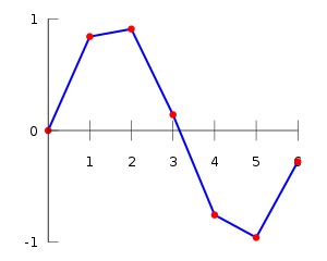
• Linear interpolation is a method of curve fitting using linear polynomials to construct new data points within the range of a discrete set of known data points.
  • E.g., estimating the value of a function between two known values
• Formula:
  • $y = y_1 + (x - x_1) \frac{(y_2 - y_1)}{(x_2 - x_1)}$
  • $p$ = point to interpolate at $(x, y)$
    • $x_1 < x < x_2$
    • $y_1 = f(x_1)$
    • $y_2 = f(x_2)$ ...
• Formula for approximating a function:
  • $p(x) = f(x_1) + (x - x_1) \frac{(f(x_2) - f(x_1))}{(x_2 - x_1)}$
  • https://en.wikipedia.org/wiki/Linear_interpolation#Linear_interpolation_as_an_approximation