5. Getting Started!
The tariff analysis tool is designed to assist stakeholders to investigate how different tariff structures impact on the expected bills of different types of residential consumers. The tool offers a range of different analysis and result visualisations as described in this section. In summary the tool allows users to:
- Create projects and add analysis to different projects for later referral
- Choose from the existing load profiles (more than 5000 annual household load profiles)
- Filter the load profiles based on the available demographic information
- Import new load profile and demographic information
- Visualise the individual and aggregate load profiles using multiple methods including seasonal pattern, peak analysis, annual energy distribution, daily interquartile range, etc
- Apply the network tariffs available in the tool (60+ tariffs for different Australian States) to calculate the annual bill based on any subset of the load profiles
- Apply the retail tariffs available in the tool
- Modify the parameters of the tariffs to investigate the impacts on annual bills
- Investigate different components of the network bill (DUOS, TUOS, and NUOS) to calculate the revenue for different sectors (distribution, transmission, etc). This can also be done for the retail component where retail tariffs are available
- Adjusting the network peak time to see the impact on the tariffs based on the coincident peak demand
- Create different types of new tariffs including, flat rate, time of use, block usage, demand charge, etc
- Compare the results of multiple analyses in different visualisation platforms including single variable comparison, dual variable comparison, and individual cases
- Export the figures, and copy them into clipboard to incorporate in any report
- Export the results to excel file to do further analysis on the results outside the tool The rest of this section introduces different parts of the tool and gives instructions on how to work with the tool.
The TDA tool does not need to installed in your computer. You only need to run the tool and do the analysis. In order to import and export the data properly (such as selecting load data, exporting result, etc), you need to keep all contents of the TDA folder. If you save a project, or create a new load/tariff, it will be also saved in this folder. Windows users need to run the TDA.exe and work with the tool. But if you are using Mac, each time you open the software, it will ask you to locate the TDA folder in your computer. Once asked, you should find the TDA folder and open it and then work with the tool.
While you are working with the tariff tool, you may want to save your current session for later referral. You can “save” the project, and later “open” the project with your saved analysis loaded in the tool. You can also delete any of the previously saved projects. You can also restart the tool to delete all analysis currently displaying on the tool and restart your analysis. If you do not save the project, the project name will be shown as “undefined” and any analysis will be lost if you close the software. Restarting the tool does not delete any project or load data. But any analyses after the last save will be lost. You cannot restore any deleted projects!
Using this menu, you can import new load data, delete any of the existing load data, or restore to the original load data list. Section 5.4 explains how to import new load data. You can also define the network load as described in 5.5. We will provide new load data as it becomes available. In that case you can just download the load data (.mat file) and put it in the “Data” directory in the TDA folder. You can check for new updates by clicking on Menu: Help > Check for Update. You can also set the maximum amount of missing data allowed as well as the down-sample rate (where a smaller percentage of the sample can be randomly selected, as described in section 5.3). By restoring the load data, any new load data you created will be lost.
You can create new tariffs, obtain the excel file with all the parameters of all the tariffs used in this tool and also reset the tariff lists to the original list of tariffs. We will provide new tariff data as it becomes available. As new tariffs are generally introduced every year, new versions will be made available and you can download them and copy them in the “Data” directory in the TDA folder as advised in the update page. NOTE. By resetting the tariffs, any new tariffs you have created or modified will be lost and this cannot be undone!
You can export the figure currently showing in the tool (ctrl+E) or copy it to the clipboard (ctrl+C) so you can paste it in another document, email, etc. You can also export the data directly from the figure (ctrl+D) or export the whole case’s results as described in following sections.
Using this menu, you can specify some options such as ‘ask to name new cases’, ‘confirm before exiting the tool’, and ‘confirm before deleting some items’.
The option “About” provides information about the software. You can click on any of three options (CEEM webpage, Researchgate project page, or GitHub page) for more information, updates, and comments about the software. You can also open the instruction file via the “Users’ Guide” option and give feedback on the software, and subscribe to receive the latest news of the software. Please note that due to some issues with internet security programs, the options to send feedback or subscribe may not work properly in some cases. If you experience this issue and receive any error message, or if you successfully submit your request but don’t receive an email confirmation, please send an email to n.haghdadi@unsw.edu.au with your feedback or subscription request.
You can select one of the existing load datasets in the tool by choosing from the dropdown list as shown in Figure 1. Before importing, you can specify the maximum allowed missing data from the menu: Load > Maximum Allowed Missing Data (%). The default value is 5%, which means only homes with less than 5% missing intervals will be loaded. You can change this each time you select a new load. You can also down-sample the load data to speed up the calculation by selecting from menu: Load > Down-sample Users (Random Selection). The default option is 100% (full data) which loads the whole dataset. 50% means randomly selecting 50% of the homes, and so forth. Please note, each time you press “Set”, a new subset will be randomly selected, so multiple selection of one load dataset with the same down-sample value will result in different users being selected.
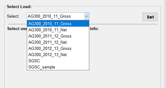
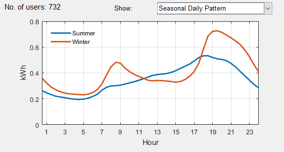
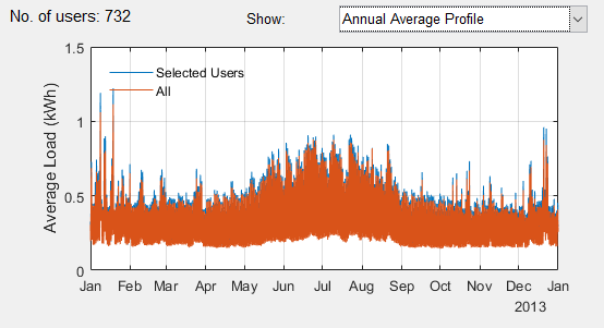
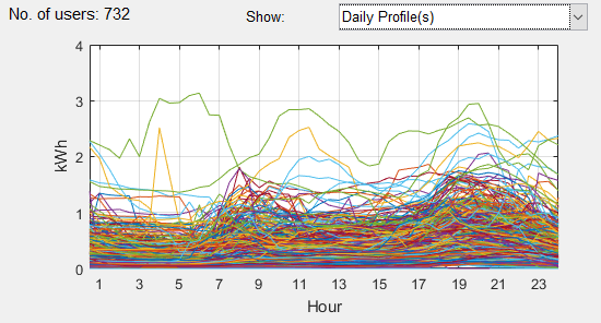
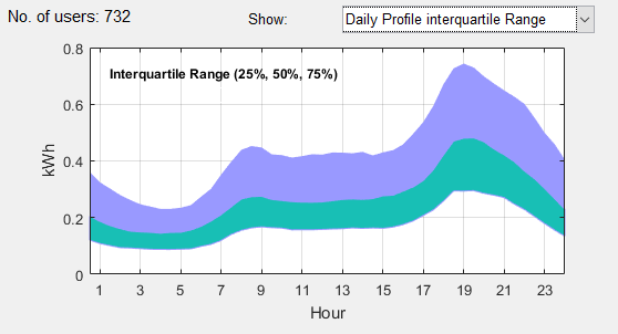
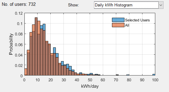
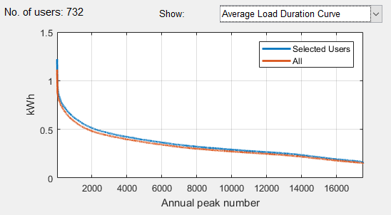
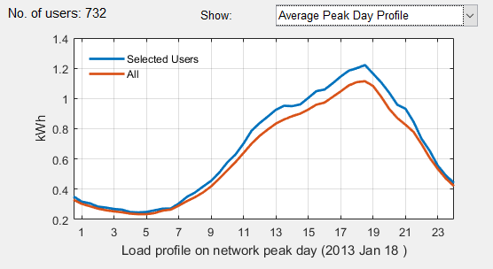
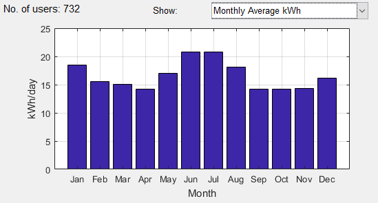
You can see the number of homes loaded into the software in the below part of the “Select Load” panel. Each dataset can be selected, and the analysis can be done based on the whole or part of that dataset which is grouped by demographic information. If the demographic information is available for any load data, it will be shown below the dropdown list (see Figure 1). You can then filter the load based on any part of the demographic information. The number of homes obtained with any particular filter is shown. There is also a set of diagrams which show the individual or aggregate behaviour of the selected load profile. So, you can see the load pattern while selecting the filters. In some of the figure options, you can see and compare the filtered load (by missing data%, down-sampling, and demographic filters) with the whole dataset. This is particularly useful if you want to check if important information (e.g. load profile on a peak day) is similar in the down-sampled load and the whole dataset. If you see a significant difference you may load the demand data again to randomise the users and load a new group. You can change the diagram type from the dropdown list. You can choose the following options (Figure 2):
- Annual Average Profile
- Daily Profiles
- Daily Profile Interquartile Range (25%, 50%, and 75% of load)
- Daily kWh Histogram
- Average Load Duration Curve (sorted aggregate load profile in kW in descending order)
- Average Peak Day Profile (daily pattern in highest aggregate peak day)
- Monthly Average kWh
- Seasonal Daily Pattern (average daily load pattern in summer and winter months)