Walk Through

Welcome to stokesim, a lightweight simulator for air/marine-crafts (planes, copters, boats, submarines...) operating simultaneously in a single environment. Each craft can have any configuration of thrusters (motor-driven propellers), control surfaces (servo-driven thin rigid plates), and sensors (IMU, magnetometer, pitot, etc...). A multipoint computational model is used where the craft and its control surfaces are treated as mechanically coupled bodies independently interacting with the surrounding fluid. Fluid interaction is based on incompressible momentum fluxes. Some may describe it as a simplified panel method.

This simulator is focused on utility for roboticists. It captures a large amount of nonlinear phenomena even when constant aero-coefficients are used, so it can be more readily leveraged by modern motion planning and control algorithms. Many vehicles can be simulated simultaneously in real-time (or faster) for swarm algorithm development. This simulator is not meant to capture very fine details like non-rigid structural dynamics or flow-field effects like wake turbulence; it is not meant to be an airframe design tool. It is a GNC and AI development tool with higher fidelity vehicle and environment physics than are provided by similar tools.

This walk-through is intended to familiarize you with the code-base and interface, conventions, etc. Here we will explain how to use stokesim while simultaneously tracing through the relevant implementation details. Warning: There are a few features not discussed here.

Architecture

All namespaces correspond exactly to the actual directory structure of the code base. For example, all code in include/stokesim/physics/actuator_types/ will be scoped to the namespace stokesim::physics::actuator_types. As another example, the class declared in include/stokesim/io/plugin.h is stokesim::io::Plugin.

Stokesim is object oriented. The attributes of each individual class are always organized into the following semantic groups (denoted in the code by Doxygen comments):

• Provided: Immutable variables that replicate the information obtained from the constructor arguments. For example, the Geoid class must be provided with the semi-major axis and flattening factor in its constructor data, so these variables are stored as-is in the Provided attributes group. As we will see, the constructor generally just takes a YAML file, so the list of Provided attributes clarifies what data is expected to be in that YAML file.

• Derived: Variables that are computed based on the Provided attributes or later calculations. For example, in some of its methods the Geoid class needs to know the semi-minor axis, which can be computed from the semi-major axis and flattening factor, but it would be inefficient to recompute it at every method call, so it is stored as a Derived attribute.

• Utilities: Methods that don't modify any of their object's attributes. For example, ecef_from_enu(...) in the Geoid class computes the ECEF coordinates corresponding to given ENU coordinates but does not modify any attributes. Utilities are essentially calculators that can be used by programs that receive a constant reference to the object (like the plugins discussed later).

• Types: Structures defined within the class because their purpose is specific to the class. For example, all of the classes in the physics namespace have their own Type attribute struct called Cmd which acts as a container for the information that can be passed into their respective update functions.

• Core: Private methods and attributes that are only reachable by the Simulator class. Any Core methods can and will modify other attributes. The classes in the physics namespace put their constructor in this group for reasons discussed later.

• Access: "Get" and "set" functions for accessing private variable attributes. This group is unique to the Simulator class as it is the only externally accessible class that needs such restrictive access.

Besides these semantic groupings and some other superficial details, most of the classes have very little in common, meaning inheritance plays an oddly small role in the overall architecture. Instead, the architecture is a "container tree" as shown below.

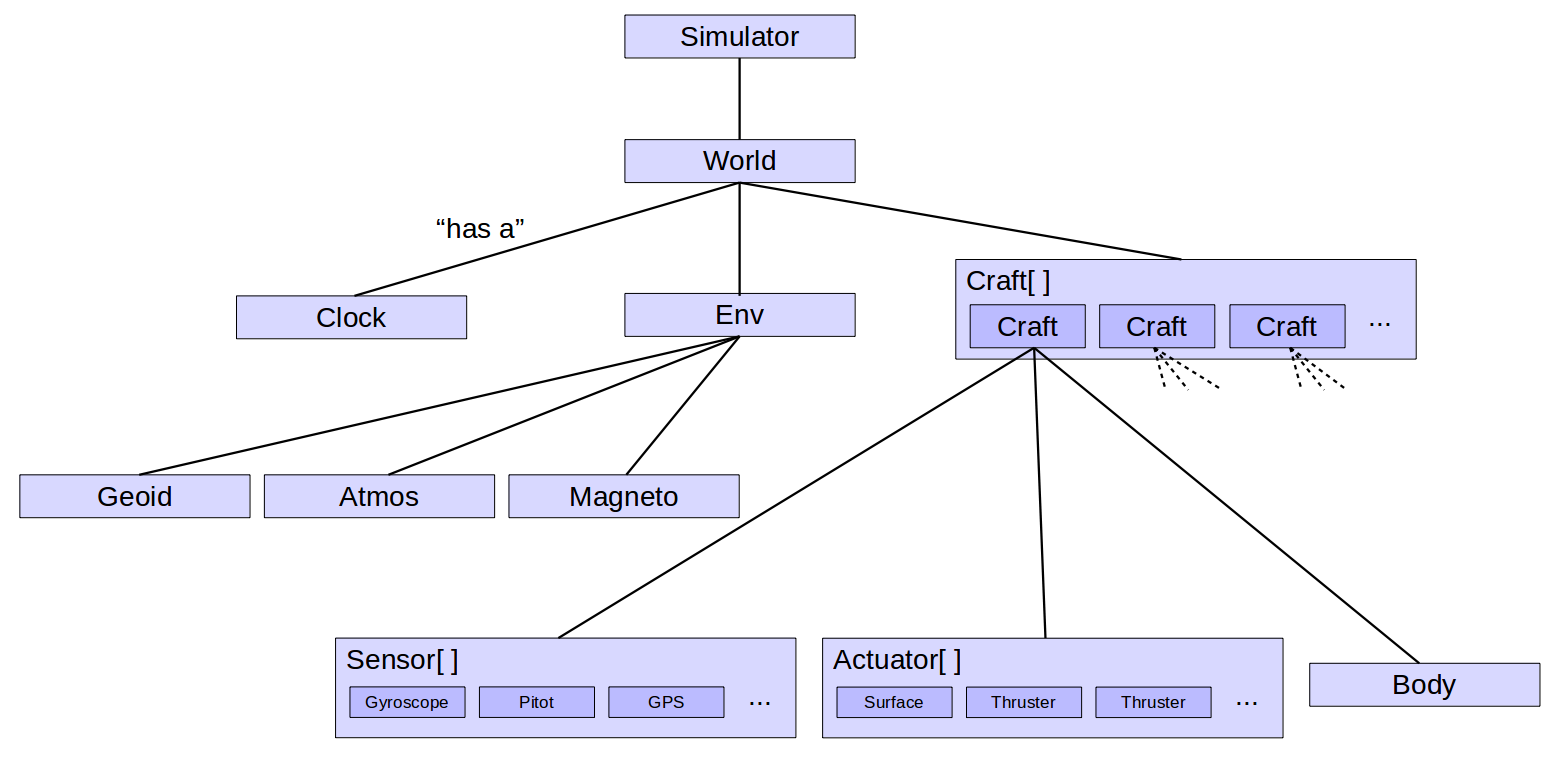
In the above diagram, each line represents a "container-contained" relationship. The container class (placed higher-up) has an instance of the contained class (placed lower down). At the same time, the contained class has a pointer to its container. Since the pathways are bi-directional, code executed from within any node in the tree can reach data anywhere else in the tree.

For example, from within a method of the Body class, we could reach the current integration timestep as this->craft->world->clock.dt. That is, any instance of Body (pointed to by this) has a pointer to the Craft that contains it (called craft), which has a pointer to the World that contains it (called world), which has a Clock attribute (called clock), which has a numeric attribute called dt.

Some classes contain an arbitrary number of another class, like how a single World can contain many unique Craft instances. The diagram represents this generally, but the specific mechanism for this is the type Dict defined in common.h to be a std::map from a std::string to some class. So the diagram is implying that a World will have a Dict of Craft called crafts.

For a more user-oriented example, suppose your current program execution has access to a World object called world. You could reach the center-of-mass position of a Craft named "cool_plane" as world.crafts.at("cool_plane").body.pos. That is, world being an instance of World will have a Dict of Craft called crafts with key "cool_plane" corresponding to a Craft value that has a Body called body with a numeric attribute called pos.

Inheritance is used where polymorphism is needed. This is currently only the case for sensors and actuators. There are a variety of "sensor types" and "actuator types" that inherit from the Sensor and Actuator base classes respectively, so that a Craft can have an arbitrary number (including zero) of any kind, uniquely configured. The code for these base classes (as well as the rest of the code base) is well commented and the currently implemented derived classes act as good examples of how you might implement your own additional sensor or actuator (and then make a pull request to become an awesome stokesim developer).

At this point you should get the gist of how the code is organized and how data / methods can be reached if you were to have access to some objects in the stokesim namespace. Now we can discuss making and using those objects for simulation.

Interface

All of the classes in the stokesim tree have private constructors except the Simulator class. However, each class declares its container to be a friend (in the C++ sense). This means that only Simulator can construct instances of Clock, Env, and Craft, while only Env can construct instances of Geoid, Atmos, and Magneto, and so forth. The end result is that the entire tree of objects branching from a single Simulator can only be constructed all at once, from top to bottom, in a depth-first fashion. For example, it is not possible to construct just a Craft in isolation. This restriction makes sense because in general, any of the methods in Craft can use their object's world pointer to climb the tree for some other necessary data. If the rest of the tree doesn't exist, that would be nonsense, so stokesim enforces its existence.

So what is needed to construct a Simulator? Well, if we look at simulator.h, we see the following under the Provided attribute group:

bool const        realtime;
Escal const       end_time;
physics::World    world;
...

So we can expect that the Simulator constructor requires at least a bool, an Escal (defined in common.h), and a World. But we won't be able to pass in a World since we cannot construct one. Instead, we must pass in all the things needed to construct a World so the Simulator can do it for us. If you look at the Provided group for World, you'll find that it needs some basic data types as well as a Clock, Env, and Dict of Craft. You'll end up recursing your way down the stokesim tree compiling a long list of what is necessary to construct the entire stokesim tree.

Meanwhile, the Simulator constructor takes just one argument: a YAML::Node called config. The structure of the YAML data should have a 1:1 correspondence with the stokesim tree of Provided attributes. Here is a pseudo-example of a YAML file that encodes the data that should be in config:

#### myconfig.yml
#### This data will be read into your program at runtime using YAML::LoadFile
#### and then it will be provided to the constructor of a stokesim::Simulator.
#### Each key-value pair below corresponds to a Provided attribute.
#### THE MEANING OF EVERY QUANTITY HERE IS IN A COMMENT NEXT TO ITS DECLARATION IN THE C++ CODE.
##################################################
realtime: true
end_time: 100
world:
    clock:
        dt0: 0.001
    env:
        geoid:
            a: 6378137
            c20: -0.00108263
            enu0_lla: {alt: 1, lat: 42.493759, lon: -71.674338}
            f: 0.0033528106647474805
            u: 398600441800000.0
            w: [0, 0, 7.292e-05]
        atmos:
            ...
        ...
    crafts:
        cool_plane:
            battery0: 500
            body:
                ...
            ...
        awesome_submarine:
            ...
    ...
...
##################################################

The Simulator constructor will read the data it personally needs from this YAML and pass the rest down the tree as the constructor for each node is called recursively.

Say you want to run a simulation with 200 different Craft objects having some attributes in common but some different. It would be very tedious to write the above YAML file by hand, so it is recommended that you script its generation. Python is probably the best choice for this, being as it is so friendly with YAML. In the config/ directory you will notice executables with the extension .gen. Anything with the .gen extension in config/ will be executed when cmake is invoked, but of course you could execute them manually any time. All they do is write a .yml file which can then be used for a Simulator. Being as many things are consistent across scenarios (like parameters specific to the Earth), reusable portions of the overall config generation scripts are broken-out into the directory config/models/. This workflow is just a suggestion though. How you get the YAML data from your head to the Simulator constructor is totally up to you.

The YAML data configures everything about the initial simulation state, from atmospheric parameter values to the initial states of all the robots. In essence, it describes a scenario. You then construct a Simulator object with this scenario, call its simulate() method, and you're done. This is actually all main.cpp (which compiles to the executable stokesim) really does. It takes as a shell argument the name of a YAML file that has your desired scenario, loads it via yaml-cpp, constructs a Simulator with it, and calls simulator.simulate(). At that point the simulator has the main loop and does its thing until the termination criteria (remember end_time?) is met or something external triggers a kill. (Under the hood, the simulator is just successively and recursively calling the update method of each node in the tree).

But generally, we don't just want to run a simulation. We want to interact with it! That includes even recording intermediate results, say to make a log file of all the craft positions over time. For this we need something that runs interwoven with simulator solution advances. Such programs are referred to here as plugins.

In plugin.h an abstract base class called Plugin is declared. Classes that derive from Plugin must implement two pure virtual functions: configure and work. The configure function will get called once at the beginning of the simulation, and the work function will be called throughout the simulation at a specified frequency. In the diagram below, the plugin happens to be running at 1/(4dt) Hz.

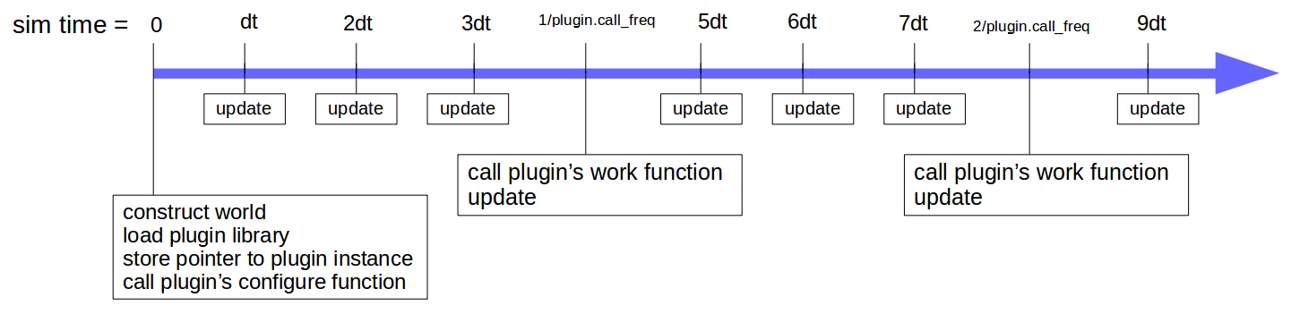
A Simulator is Provided with an arbitrary number of these Plugin-derived classes. To keep the overall configuration architecture consistent, the Simulator is still responsible for constructing each Plugin that it will hold- you only have to give it the constructor arguments within the same YAML as everything else.

In the example below, we intend for our Simulator to run two plugins interwoven with the simulation process. They are named "cool_plane_logger" and "thing_doer".

# myconfig_with_plugins.yml
...
world:
    ...
plugins:
    cool_plane_logger:
        bin_file:   "/path/to/logger.so"
        call_freq:  100  # Hz
        craft_name: "cool_plane"
        log_file:   "/log_folder/cool_plane_log.txt"
    thing_doer:
        bin_file:   "/path/to/some_other_plugin.so"
        call_freq:  60  # Hz
        ...
    ...

When the Simulator goes to construct the plugin named "cool_plane_logger", it will dynamically link to the library logger.so where it is assumed you have defined a Plugin-derived class (probably named Logger). It will try to call a function called create() that should return a pointer to a Plugin (specifically, a Logger instance). In plugin.h there is a macro EXPORT_AS_PLUGIN(CLASS) that ensures the create() function stokesim needs will be there. To clarify, this is what the source that compiles to logger.so might look like:

// logger.cpp which will be compiled to logger.so
...
#include "stokesim/io/plugin.h"
class Logger : public stokesim::io::Plugin {
    std::string craft_name;
    std::string log_file;
    bool configure(YAML::Node const& config, stokesim::physics::World const& world) override {
        ...
    }
    Output work(stokesim::physics::World const& world) override {
        ...
    }
}
EXPORT_AS_PLUGIN(Logger)

Note that the attributes bin_file and call_freq are not declared in Logger because they come from Plugin since all plugins require them. For a full example, check out the actual logger plugin.

The configure function will have access to all the YAML data under the corresponding plugin's name, as well as a constant reference to the initial World (in case any of the plugin's behavior depends on the initial state of the World). The work function takes a constant reference to the current World and returns a Plugin::Output which will be described shortly. From a plugin's perspective, the World is read-only. This is why it is okay that nearly all of stokesim's class' attributes are public.

Plugins for stokesim are coroutines in a completely synchronous architecture- there is only one thread by default. If a plugin's work function hangs, the whole simulation will hang. However, nothing stops your plugin itself from starting other threads. For example, suppose you wanted to write a visualizer plugin, but your graphics take a while to process. You may write a work function that starts drawing the current scene in a new thread (or sends the relevant World data out to some other process) and then just bypasses until the thread finishes.

It is clear how and when a plugin will receive data from the simulator (i.e. the constant reference to the World passed into the work function), but how can the plugin respond to the simulator in a way that affects the simulation? This is where the return value of work, a Plugin::Output comes into play. Output is a struct that contains some data relevant to the Simulator as well as a World::Cmd. The World::Cmd has some data relevant to the World as well as a Clock::Cmd, Env::Cmd, and Dict<Craft::Cmd>. Opening up all the Cmd structs will take you down the stokesim tree again.

All Cmd structs default to values that make them irrelevant to their corresponding classes. So if your plugin just returns a default as return Output(); then in essence no information is being sent back into the simulator. You would expect this from, say, a logger plugin. However, an RCPilot plugin might want to send actuator commands into the simulator. Suppose you wanted to command an RPM to the Thruster Actuator named "left_engine" attached to the Craft named "cool_plane". You can't modify anything in World directly from your plugin's work function, but you can return your desire in the Output. In the example code below, we set that actuator command and also double the simulation timestep for example purposes:

Output RCPilot::work(stokesim::physics::World const& world) override {
    ...
    Output output;
    output.world_cmd.craft_cmds["cool_plane"].actuator_cmds["left_engine"].values["rpm"] = ...;
    output.world_cmd.clock_cmd.dt = 2*world.clock.dt; // not that an RC pilot would actually do this
    ...
    return output;
}

You couldn't modify the world.clock.dt directly because plugins only ever get const access to the World. That is, you couldn't even compile world.clock.dt *= 2;.

Theory

Stokesim models the planet as an oblate spheroid. This has implications for the conversion between geodetic coordinates (latitude, longitude, altitude) and local coordinates as well as for the calculation of gravity. The parameters defining the planet shape and rotation rate are configurable (very little in stokesim is hard-coded), but generally we want to simulate Earth, so the WGS84 Earth parameters are provided in config/models/earth.py.

Stokesim follows the robotics convention of East-North-Up (ENU) for local world-fixed coordinates and forward-left-up (FLU) for body-fixed coordinates (i.e. for coordinates fixed to crafts and their sensors and actuators). By "follows the convention" it is meant that, unless otherwise specified, those are the coordinate systems of choice. However, the Geoid class provides all the necessary Utilities to change a given positional vector's coordinate system. For example, conversions to Earth-Centered-Earth-Fixed (ECEF) and North-East-Down (NED) are available as functions, as well as to Earth-Centered-Inertial (ECI) using the current sim time. The actual rotation matrices for these conversions are also exposed for transforming velocities and accelerations (it is up to the user to implement the exact conversion desired being as various angular velocities and accelerations can come into play).

Stokesim models the static atmosphere according to the ISA relations. Again, the various parameters that make the model fit to Earth are provided in config/models/earth.py. The wind model is not based on any global atmospheric data however. The wind velocity at every point in space is modeled as an Ornstein–Uhlenbeck stochastic process in coordinates local to that point. So if you set the mean value stokesim::physics::Atmos::wind_mean to [10, 0, 0] then, on average, the wind will be blowing 10 m/s East where East is relative to the point you are calculating the wind at (using the function stokesim::physics::Atmos::wind_at_lla). In other words, the wind's characteristics wrap around the geoid. The wind velocity is computed as the mean plus a turbulence term, which is the (zero-mean) OU stochastic process. The turbulence is driven by turb_taus (time-constants for the tendency to return to zero) and turb_covar (covariance matrix for the integrated noise).

The magnetosphere uses the NOAA's World Magnetic Model, which approximates the planet's magnetic field with empirically-fitted spherical harmonics. The magnetosphere currently only impacts the readings of the Magnetometer Sensor class.

Ignoring actuators and sensors, each Craft is modeled as a single 6DOF rigid-body. The usual Newton-Euler equations apply. External wrenches come from the surrounding fluid (drag, buoyancy), the actuators, and fictitious effects due to the equations of motion being written in a planet-fixed frame (the planet rotates). The drag force vector in body coordinates is computed as,

force_drag = -density_com * areas.cwiseProduct(Cp1*vel_cp + Cp2*(vel_cp.cwiseAbs().cwiseProduct(vel_cp)))

where,

• density_com: The density of the atmosphere at the position of the body's center of mass
• areas: Frontal, lateral, and vertical largest cross-sectional areas of the body
• Cp1: A 3x3 matrix of "drag coefficients" that get multiplied by a velocity
• vel_cp: The velocity of the body's center of pressure relative to the wind
  • vel_cp = vel - ori_inv*wind_com + avel.cross(cenpres)
• Cp2: A 3x3 matrix of "drag coefficients" that get multiplied by a signed velocity-squared (i.e. |v|v)

The torque due to drag is the cross-product of the COM-lever-arm to the center of pressure and the drag force, plus an extra term that directly dampens angular velocity,

torque_drag = cenpres.cross(force_drag) - density_com*Cq*avel

This wrench really accounts for both drag and lift; it is the resultant of the incoming constant-density flow being deflected according to the relative cross-sectional areas of the body. To understand this, consider a simple 2-dimensional version with only Cp1.

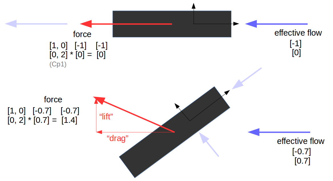
The relative sizes of the values on the diagonal of the drag matrix control how lift and drag vary with angle-of-attack. A body with a big belly but narrow nose will generate more lift when tilted as shown, because those areas factor into the drag matrix (stokesim keeps that dependence explicit by multiplying by said areas). Another way to view this is that the flux of the incoming flow (velocity with density) through the principle cross-sections of the body are what generate the net fluid-interaction force. Stokesim executes this idea in three dimensions. A variety of UAV papers use this model, and it is ubiquitous for AUVs.

It is worth noting that if you put values in the off-diagonals of the drag matrices, the body can generate lift even at zero angle-of-attack. This can model wings with nonzero incidence, or the effect of airfoils / non-prism shaped bodies. It is also worth noting that by having one term for linear dependence and one term for quadratic dependence on velocity, the relative magnitudes of their drag matrices can model where the flow regime changes from linear to quadratic (consider a plot of ax + bx^2). Overall, this fluid interaction model can reconstruct the majority of prominent geometry-driven flight phenomena. The unknown parameters involved can be estimated through experiment or even hand-tuned based on expected performance metrics.

To handle the effects of arbitrary control surfaces, each control surface is treated as a body just like above, rigidly attached to the main craft body. That is, the drag wrench for each control surface is computed (independently), and then summed up (with regard for the various lever-arms involved) to compute the total wrench due to all the control surfaces. To simplify matters slightly, being as control surfaces are generally very thin, they are only considered to have two nonzero dimensions (and thus only one nonzero area for which the fluid flux generates force on). The pose of the control surface relative to the main craft body is adjustable using a simulated servo that can rotate the surface about an axis at a limited rate. Non-actuated control surfaces like tail fins and such can be modeled as control surface actuators with 0 min and max angle limits.

Thrusters can be commanded to achieve a certain RPM (with delay due to limited angular acceleration). The thrust force generated is a quadratic function of the current RPM. The thrust force also drops off with airspeed (along the direction of the thruster) squared. The thruster also exerts a back-torque on the body proportional to the thrust it is generating. As usual all the coefficients governing these relationships are configurable, and as with control surfaces, an arbitrary number of thrusters can be attached to a craft with arbitrary poses. The sum of the thruster wrenches takes into account their placement.

The various sensor types are modeled in the usual ways done in the robotics community, including temperature-dependent walking biases, etc...

Since actuators and sensors can be attached at arbitrary poses, there are a number of craft-fixed coordinate systems to keep in mind. The diagram below gives a top-down view of an example layout.

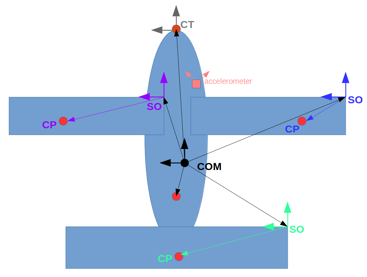
• COM: center of mass for the body
• CT: center of thrust for some thruster mounted on the nose
• CP: centers of pressure for the body as well as the various surfaces
• SO: surface origin, the origin of the coordinate system describing the initial pose of the surface

All sensors and actuators are positioned relative to the vehicle COM. However, it is recommended that in your vehicle model script you make the COM position relative to some known geometric entity and then express other positions measured relative to that point, minus the COM, so that the COM can be easily modified later.

The pose of each surface is a 3D entity, but the surface itself is an infinitely thin sheet. The 1st and 2nd dimensions of its coordinate system are the dimensions along which the surface has size. The 3rd is always the surface-normal. The definitions of these dimensions relative to the main COM-centered FLU body coordinate system are described by the following attributes Provided to a Surface,

Evec3 const origin; ///< Mounting point and origin of surface-coordinates in COM-coordinates
Equat const orient0; ///< Trim orientation of surface-coordinates relative to COM-coordinates

Unlike thrusters, a surface's coordinate system's pose changes as it is actuated. It is a simple rotation about the axis attribute. The Derived attribute orient tells you the current rotation matrix that takes the surface coordinates to the COM-centered FLU body coordinate system.

As an example, suppose we wanted to add a sweep-back angle to the left aileron in the front of the example_quadwing model. We would modify the value of orient0 in the dictionary lailf to be a slight rotation about the z direction. That would correspond to the following:

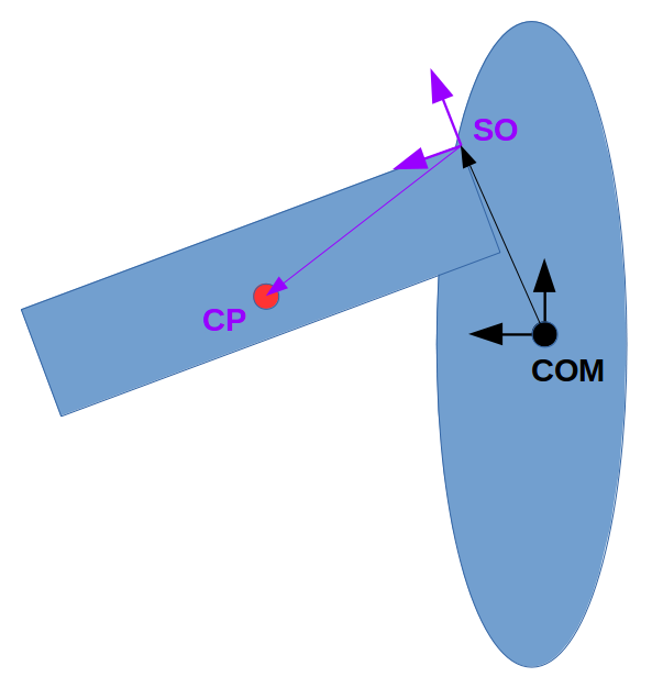
You may find it weird to place the surface coordinate system in the "upper right corner" of the surface. Don't worry, you can pose it however you want, you just have to express your center of pressure accordingly and remember that the axis of servo rotation always passes through the surface origin!