Python For Data Analysis : Seoul Bike Demand Predictions

For this project, we studied and exploited data from a bike renting company based in Seoul. The dataset which was given to us to analyse gathered data regarding the date (and info on said date such as the season, wheter it is a holiday...),the meteorological conditions, as well as the number of bikes rented on said date.

Here is the link to the dataset : https://archive.ics.uci.edu/ml/datasets/Seoul+Bike+Sharing+Demand

We placed ourselves in the position of people from the bike renting company, wanting to understand the factors playing in the demand, to be able to anticipate it. Therefore our goal was to look at all the conditions reunited (all the predicators) and study their impact on the the number of rented bikes.

Importing and exploring our data

Attribute Information

• Date : year-month-day
• Rented Bike count - Count of bikes rented at each hour
• Hour - Hour of he day
• Temperature-Temperature in Celsius
• Humidity - %
• Windspeed - m/s
• Visibility - 10m
• Dew point temperature - Celsius
• Solar radiation - MJ/m2
• Rainfall - mm
• Snowfall - cm
• Seasons - Winter, Spring, Summer, Autumn
• Holiday - Holiday/No holiday
• Functional Day - NoFunc(Non Functional Hours), Fun(Functional hours)

What we noticed

Upon importing the data, we were able to notice important aspect of the dataset :

• No NAs we present, saving us some time in cleaning up the dataframe
• The columns were improperly names (spaces, accents...), so we had to rename them

We were able to look at the type and repartition of values for all columns:

• Most of our variables were numerical and continuous, including our target (number of bikes)
• We also had categorical values included in the temporal variables
• The date variable was the only variable of type datetime, which tends to be impractical for visualizing and modeling
• There were some discreptencies in the season labels, which we corrected using the dates given to us

Graphs and observations (in the notebook and PPT)

Some plots (especially those using plotly express) may not display directly in the notebook file.

To visualize them you can either compile the notebook, or just go to the plots folder which contains all the plots we did (plots 14 to 20 may be the ones which are not displaying in the notebook preview)

What we changed

Upon exploring and visualizing our data, we made some choices in order to facilitate our work.

What we added

We ended up adding the following columns :

• day, integer from 1 to 31
• month, integer from 1 to 12
• year, integer between 2017 and 2018
• bike_affluence, categorical varaible among ("very few","few", "some", "many") (to allow us to use classification models to predict the demand, instead of just regression models)
• Moment_of_day, for a categorical representation of the hours of the day

What we removed

Upon manipulating our data, we discovered that :

• functioning_day : the functioning_day variables, which was not originally explained in the description of the dataset, was actually telling us on which days the company did not rent bikes (days when no bikes were ever rented). Since we were focusing on causes for the demand of bikes that were external to the company, whe dropped the column to focus on the other predicators.

• date : the date column would be difficult to manipulate, and we already had created new time variables (see added variables above), so we dropped it as well

• year : almost no data was recorded in the year 2017, and the great majority of our rows were from 2018. This does not mean that no bikes were rented then. By the looks of it, we most likely had little to no data recorded before november of 2017. Furthermore we only had two years to use. We figured that the year variable would disrupt, rather than help, our study and models, and since most of the data was from 2018, the loss of information would be minimal. We therefore dropped the year column as well.

• Moment of day : it was no longer usefull after visualizing the data

• dew point temperatureh : it was too correlated to temperature

• seasons : it was too correlated to month

Preprocessing the data

In preprocessing, we focused on two main tasks :

• to une label encoder and label binarizer to change our categorical predicators into numerical values
• to normalize (minmaxscaler) our numerical values to help improve the accuracy of classification models

Models

Regression Models

We started by splitting our data into a training and testing set, with the continuous variable number of rented bikes as target. The training set was composed of 90% of the dataset, and the testing set of 10%.

In order to define which regression models to use for out data, we used the lazypredict package on our training set to give us a first evaluation of all models available (using only the default parameters). Although we were unable to fully run the selection, we were left with the results for 31 out of 42 of the models evaluated. We chose the ones which had the lowest RMSE, as they would be the most accurate. This left us with the following models :

• Gradient Boosting Regressor
• Hist Gradient Boosting Regressor
• Bagging Regressor
• LGBM Regressor
• Random Forest Regressor
• Extra Trees Regressor

We also tried using a KNN Regressor and Linear Regression model, which we were familiar with, to no avail.

We then used GridSearchCV to find the best hyperparameters, which gave us :

• Gradient Boosting Regressor {'learning_rate': 0.3, 'loss': 'huber', 'n_estimators': 109}
• Hist Gradient Boosting Regressor {'learning_rate': 0.2, 'loss': 'poisson', 'max_iter': 109}
• Bagging Regressor {'max_samples': 1.0, 'n_estimators': 26}
• LGBM Regressor {'boosting_type': 'dart', 'learning_rate': 0.4, 'num_leaves': 37}
• Random Forest Regressor {'n_estimators' = 100}
• Extra Trees Regressor {'criterion': 'squared_error', 'n_estimators': 101}
• KNNR {'algorithm': 'brute', 'n_neighbors': 6, 'weights': 'distance'}
• Linear Regression

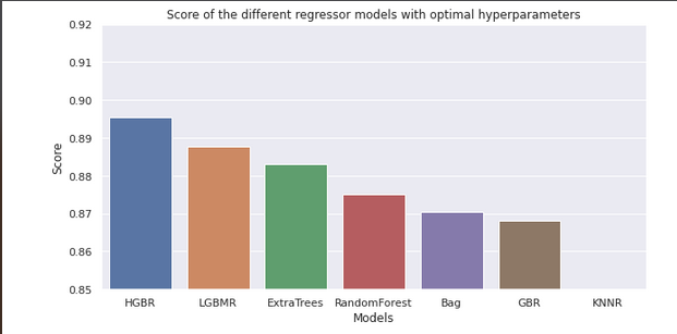
We then evaluated the score of each optimized model (comparing predicted values to observed values), and came to the conclusion that the models were, from best to worst :

• Hist Gradient Boosting Regressor (~0.89)
• LGBM Regressor (~0.88)
• Extra Trees Regressor (~0.88)
• Random Forest Regressor (~0.87)
• Bagging Regressor (~0.86)
• Gradient Boosting Regressor (~0.85)
• KNNR (~0.57)
• Linear Regression (~0.51)

To sum up the results :

Classification Models

We started by splitting our data into a training and testing set, with the categorical variable bike affluence as target. The training set was composed of 90% of the dataset, and the testing set of 10%.

We again used the lazypredict package on our training set to give us a first evaluation of all models available . We were this time able to fully run the selection, and we were left with the following models, which had the best evaluated accuracy. From most to least accurate :

• LGBM Classifier
• Random Forest Classifier
• Extra Trees Classifier

We also tried using a KNN model, which we were familiar with, to no avail.

We then used GridSearchCV to find the best hyperparameters, which gave us :

• LGBM Classifier {'boosting_type': 'gbdt', 'max_depth': -1, 'num_leaves': 35}
• Random Forest Classifier {'criterion': 'entropy', 'n_estimators': 124}
• Extra Trees Classifier {'criterion': 'gini', 'n_estimators': 122}
• KNN {'n_neighbors': 3, 'p': 1}

We then evaluated the accuracy of each optimized model :

• LGBM Classifier (~0.80)
• Random Forest Classifier (~0.80)
• Extra Trees Classifier (~0.80)
• KNN (~0.73)

API

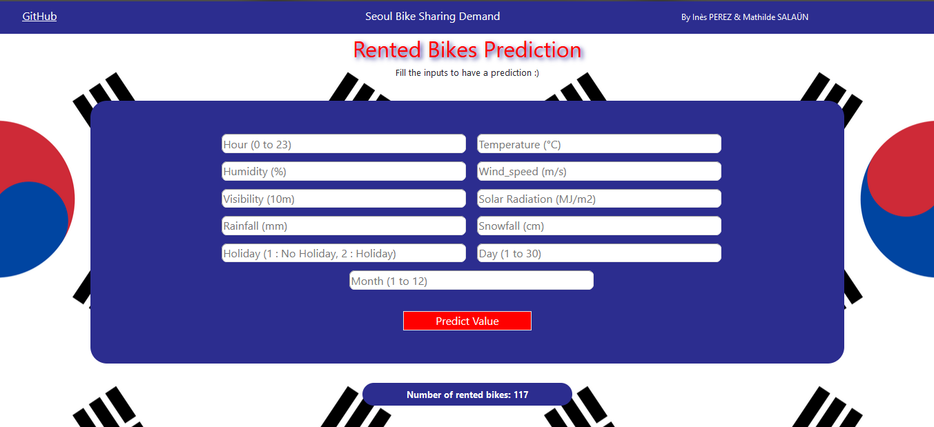
We then created an API with Flask, allowing a user to find out how many bikes would be rented in a day based on:

• the hour
• the temperature
• the humidity
• the wind speed
• the visibility
• the solar radiation
• the rainfall
• the snowfall
• the holiday
• the day
• the month

The aim is to allow professionnals to anticipate the demand for bikes based on time and on the predicted meteorological conditions.

The API was originally going to use our most accurate model, which was the Hist Gradient Boosting Regressor. However we had issues with the package sklearn.ensemble which contained the model type we wanted, as well as all of our most efficient models. We therefore had to find another model, the LGBM Regressor - that turned out to be our second best model -, which we deployed in the api with the hyperparameters {'boosting_type': 'dart', 'learning_rate': 0.4, 'num_leaves': 37} and an estimated score of ~0.89.

The finished API presents as follows :

Some room for progress

Although we did our best with the tile we had, we do have some ideas to further improve the API. We could have the user give us just a day, month and hour, deduce from our data if that date is a holiday, and by recuperating the associated meteorological data in a weather info web page, enter all the remaining parameters in the API so it can return a result. This would give less constraints to the user as he/she would only have time data to enter.

Difficulties encountered

Most of our issues came from :

• learning how to use new elements such as Flask
• running grid searches and predictions, which could be very long and sometimes never finished running
• installing and deploying packages (see problem with Flask evoked above)

What we learned

Through this project we had the occasion to learn, apply or dig into notions such as:

• detailed analysis of a dataset
• manipulation and visualization of data
• selecting relevant
• preprocessing of data
• machine learning models
• optimization of said models
• creation of an API

We will now be able to use this experience to produce even better projects in the future.