Borui Wei
This project explores the use of deep learning techniques to distinguish between two types of instruments - kicks and toms, in a drum set using sensor data. This project is inspired by the demonstration projects on Edge Impulse, where deep learning models deployed on sensors have shown the capacity to recognise a continuous sound - the runing faucet, or to respond to more complicated words with syllables.
The objective is to explore the ability of deep learning models to tell different tone colours with the help of sensors. Sometimes in music production especially electronic sound engineering, there are sounds that easily to get mixed with others, like toms and kicks. Although these sounds are engineered with rules (i.e. toms and kicks certainly have different auditory perceptions), sometimes there could be still be difficulties telling them apart by human ears. Deep learning models may 'hear' these different sounds and distinguish them in a quite different way -- by analyzing the spectrograms ('seeing' the sound rather than hearing), which may provide an innovative solution to this problem.
The project has developed an application that can be deployed on an Arduino 33 BLE sensor through the help of Edge Impulse. The application can be runned either on desktop terminal, or By deploying it on a suitable sensor, the model embedded will analyse the signal that the sensor has to intake, and returns an answer determining whether the sound clip is likely to be a kick or tom. Given an accuracy of 80%, the application is relatively trustful in classifying these 2 instruments from a drum set.
|
|
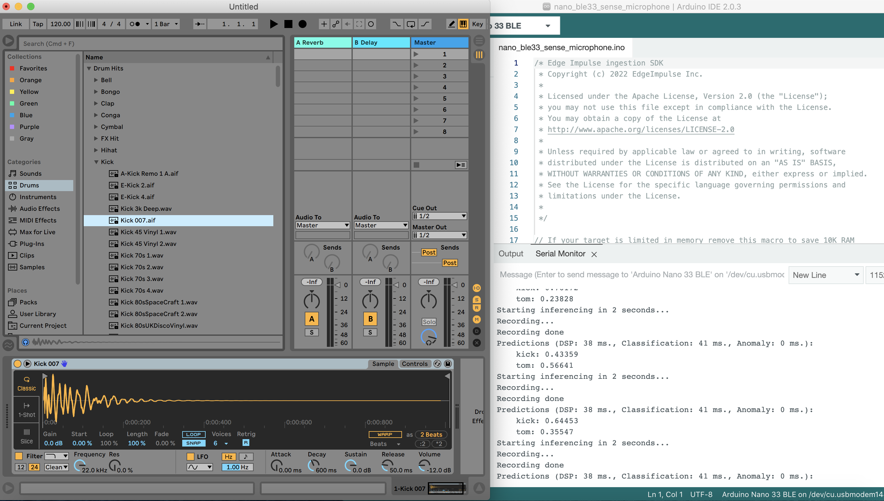
Figure 1. A demonstration of the application in Arduino IDE-- connect sensor and record the sound played by desktop. The sensor flashes differently on classification
-
How effcient are the deep learning models combined with sensors in distinguishing different electronic instruments.
-
What features in different sounds are better extracted by deep learning models? Are there any features overused and other neglected?
This application components were Edge Impulse, Arduino BLE33 microphone and the Arduino IDE. Edge Impulse, as an end-to-end development platform for building and deploying machine learning models on edge devices played an important role in linking the components together by accomplishing the following tasks:
- Generating files to update the firmware on Arduino BLE33 and make it ready for connection;
- Operating the sensor to sample data, and train-test set splitting of sampled data;
- Model building, training, and testing (with test set or live testing with new clips recorded);
- Generating model deployment solutions for Arduino sensor that can be runned in desktop terminal or the Arduino IDE.
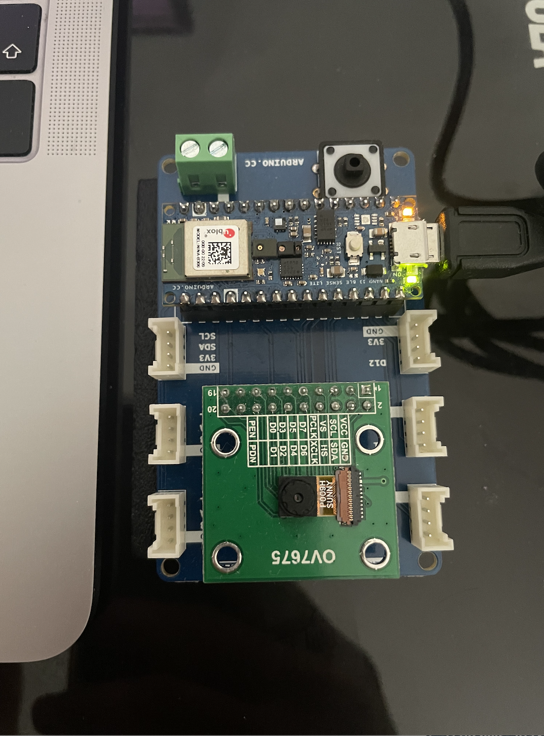
In terms of the hardwares, The Arduino BLE33 sensor that has recording functionality is required to be connected to a supportive desktop so that it can be operated through Edge Impulse in data sampling and live testing tasks, or the deployment through desktop shell command and Arduino IDE. A flow chart that illustrate the application build is shown in the flow chart below:
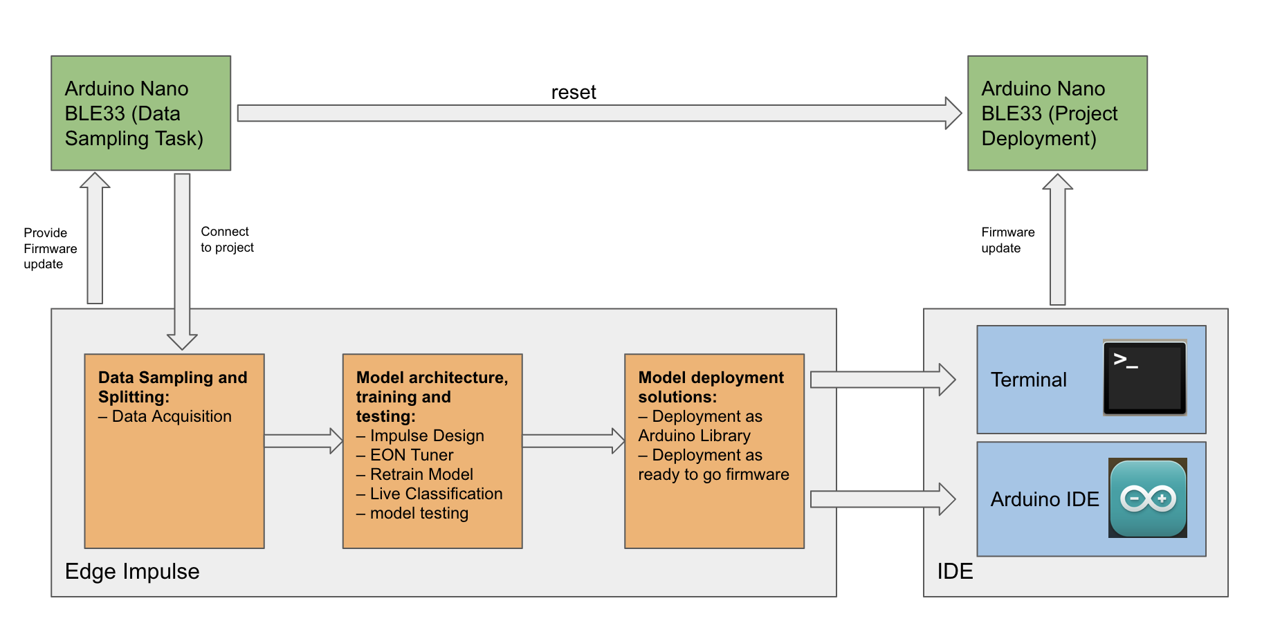
Figure 2. Application build flowchart
The system requirements where this project is developed and tested is provided as follows:
- macOS Catalina version 10.15.4
- Arduino IDE (2.0.3)
This application can be deployed and tested on Arduino BLE33 sensor in two ways:
- A ready-to-use shell application that can be runned directly on a desktop with Arduino BLE33 sensor connected. By cloning down the folder named "drum-rack-nano-ble33-sense" in this repository to local, run the 'flash-mac.command' file to install the mapplication firmware on the sensor. After the installation is finished, start up a new command window and run command:
edge-impulse-run-impulseThe application will run and log the following in the terminal on your desktop. The sound clip should be played after the 'Recording' prompt and the results are printed at the end of each classification loop:
Starting inferencing in 2 seconds...
Recording...
Recording done
Predictions (DSP: 33 ms., Classification: 31 ms., Anomaly: 0 ms.):
    kick: 0.73047
    tom: 0.26953
- A library for Arduino IDE -- By downloading the zip file named 'ei-drum-rack-arduino-1.0.2.zip' to the local. This zip file can then be included as a library in Arduino IDE.
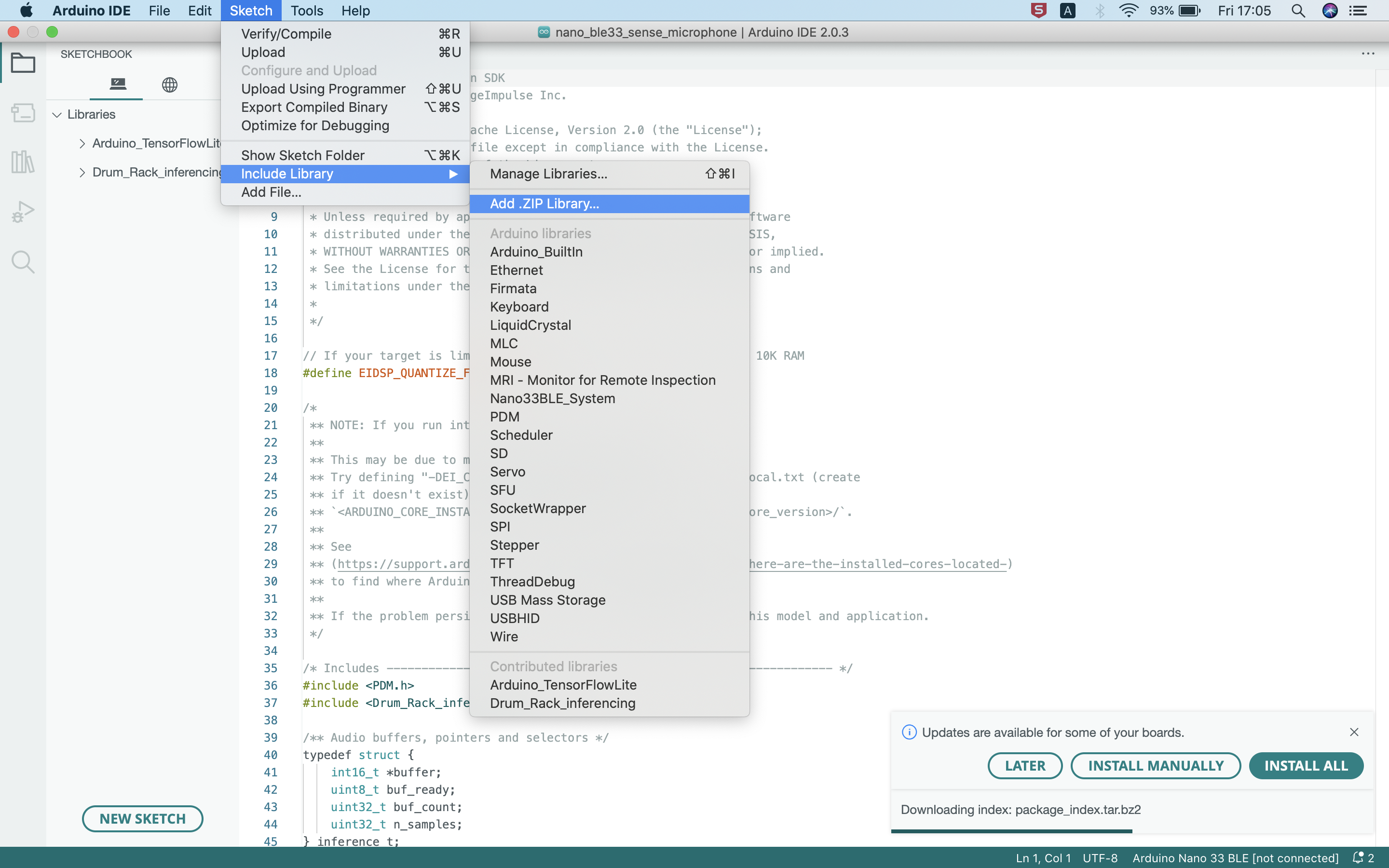
Figure 3. Include the model as library in Arduino IDE
Then download and open up the sketch file '/nano_ble33_sense_microphone/nano_ble33_sense_microphone.ino', click upload button to run the application. The output can be monitored via Tools > Serial monitor where the signal processing pipeline can be started. The 'baud rate' is recommended to be set at 115200, which indicates the data sent by the Arduino board will be transmitted at a speed of 115,200 bits per second.
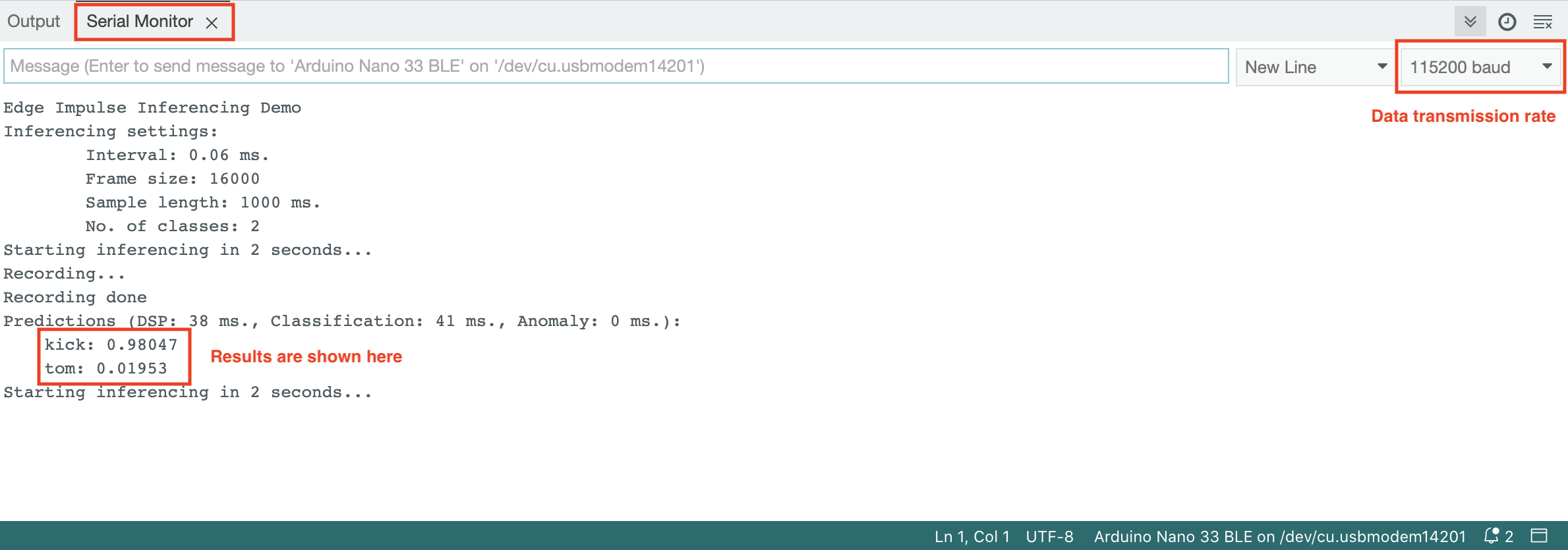
Figure 4. Run the model and monitor outputs in Arduino IDE
This option to deploy the model as an Arduino library has 2 new features: 1. The delay per inferencing loop is set as 5000ms to make the application more user-friendly. 2. The classification result can be observed through different flashing behaviours of the on board LED: It is set to flash once for 1000ms if the result is 'kick' and to flash 5 times for 50ms each time if the result indicates 'tom'.
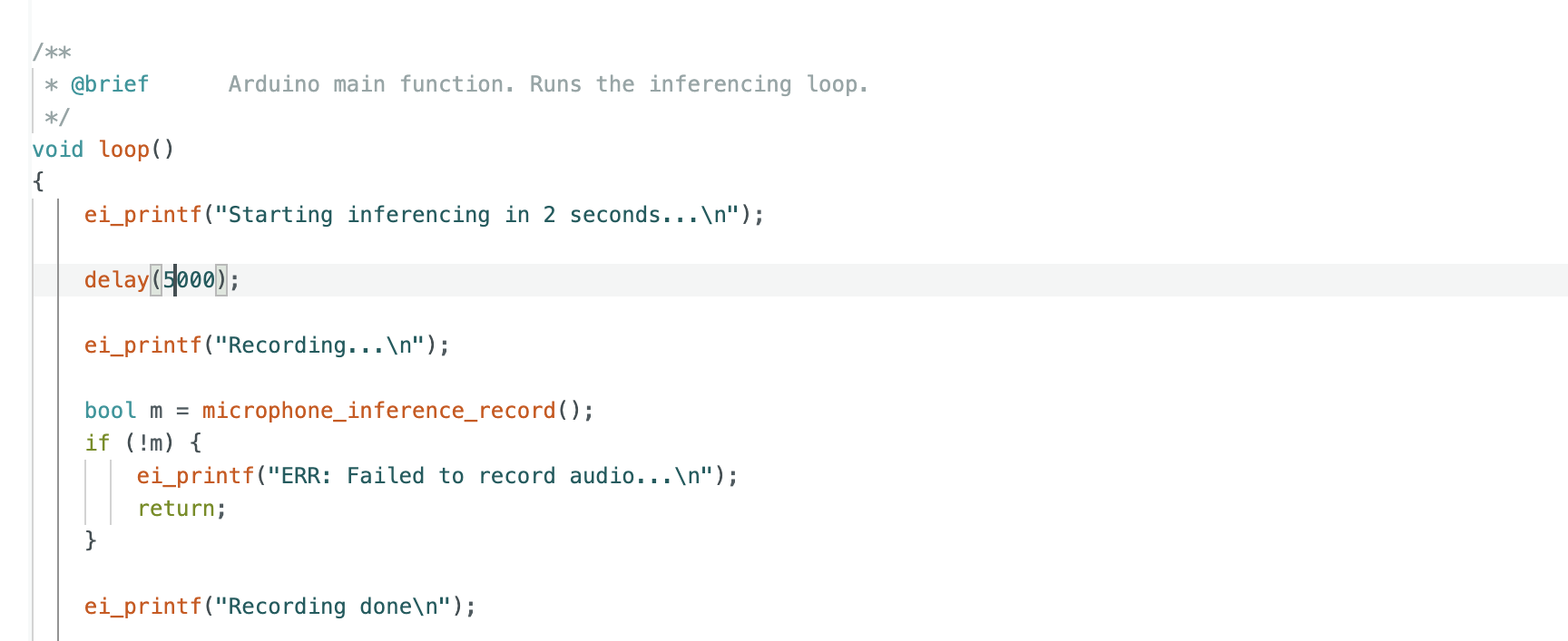
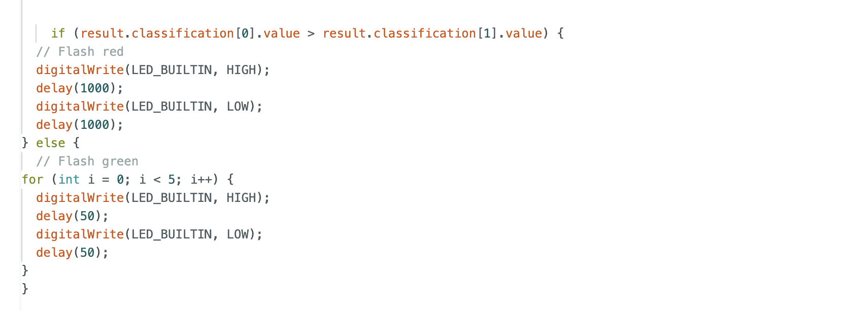
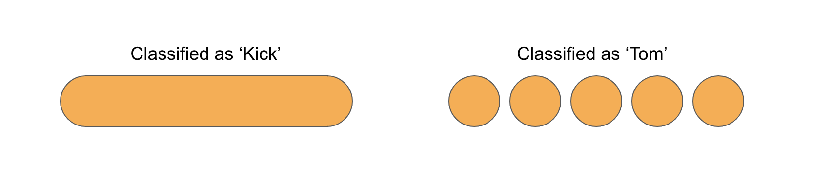
Figure 5. different LED flash pattern on classification
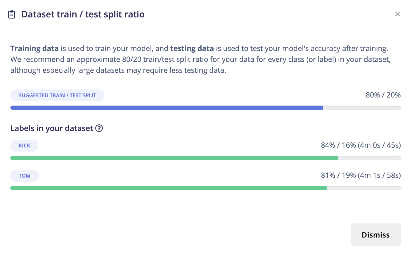
The data are sampled from mainly 2 sources: demo clips from Splice Sounds and self-contained audio sources from Ableton Live Suite 10 [1]. The sound clips labeled as 'kicks' and 'toms' are played on the desktop and recorded by Arduino Nano BLE33 built-in microphone. The signal recorded was then transmitted and uploaded to Edge Impulse platform, where labels can be given according to their orginal groups and a preview of the shapes of the signals can be presented. The data samples are collected as sound clips of 15000 miliseconds at 16000 hertz. The sampling rate is decided to satisfy the Nyquist's theorem for all samples. (for detailed information please refer to [iii]) Around 80% of the data (313 records) was splitted as training set and 20% (84 records) as test set, and in total they account for 10m10s of audio recording.
 |
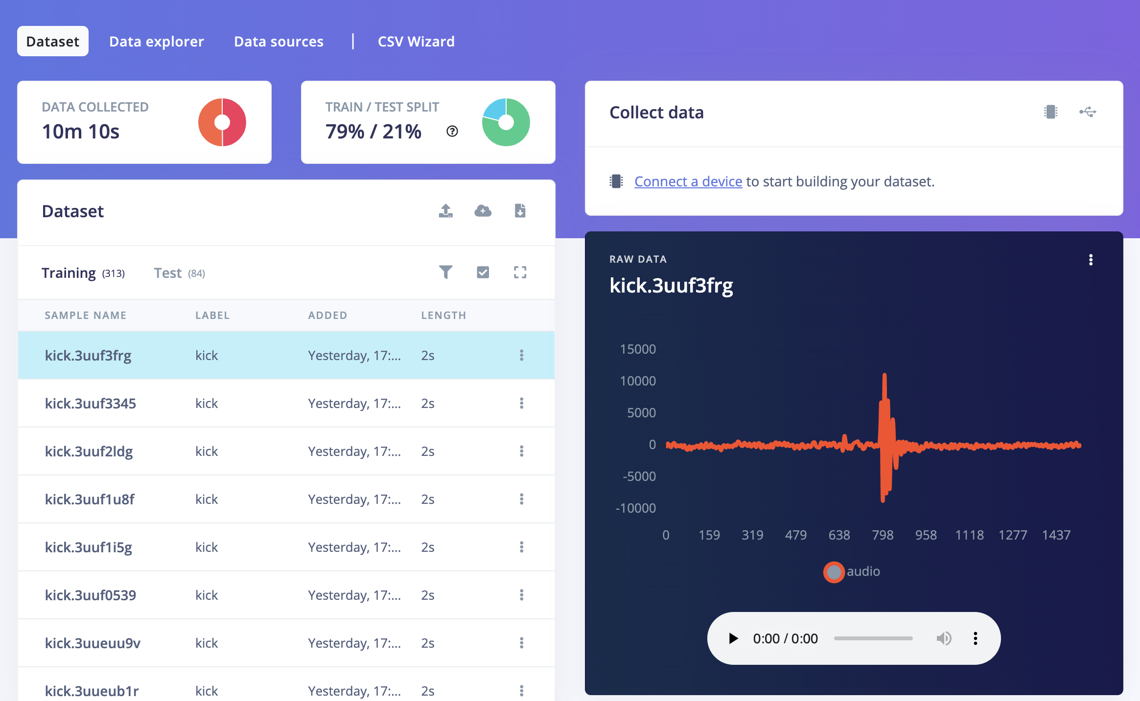 |
Figure 6. Data Sampling and train-test splitting
These latter preprocessing steps are implemented within the models building processes and are going to be introduced in the 'Experiments' section.
The model architecture chosen is a Spectrogram model with 4 1-dimensional convolutional neural network. The model requires 4 hyperparameters: Frame length, Frame stride and FFT length. Frame length was set as 0.025 second, indicating the length of segments when performing windowing over each record. Frame stride was decided as 0.025 second, meaning that the neighbouring two windows does not have any overlapping. FFT length is decided as 128, meaning that within each cycle on the frequency chart, 128 sample points are taken to represent the oscillation during the period of time within the cycle (detailed information please refer to appendix[iii]). This process of how raw data is processed through setting these parameters is shown here:
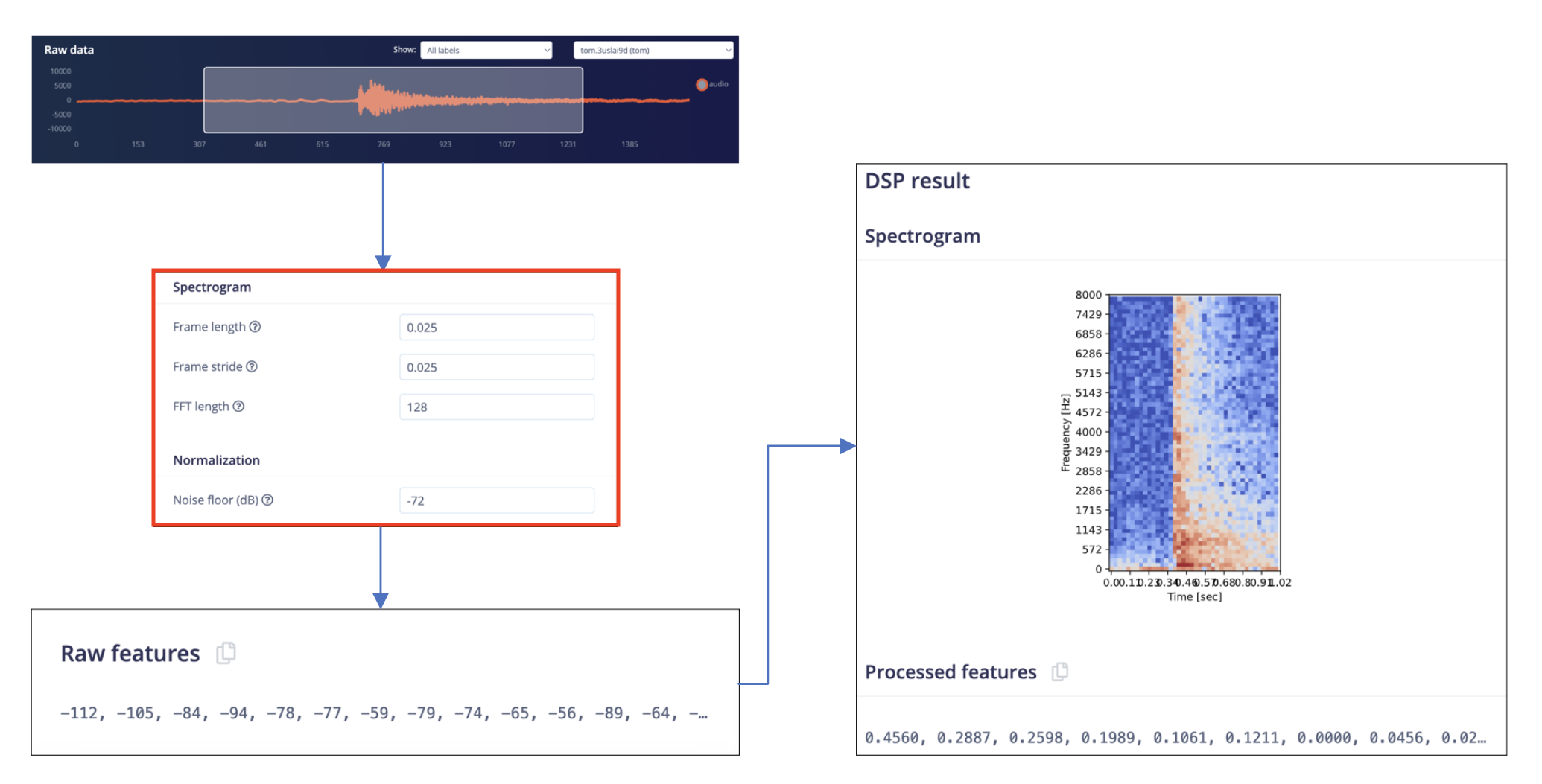
Figure 7. Data preprocessing in selected model
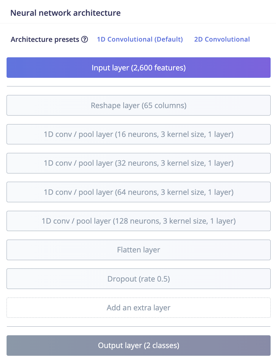
In the next steps, the preprocessed data samples are put into the neural network that is structured as shown in the image below. The 2600 features processed from the last step as the input layer was firstly reshaped into 65 columns. The reshaped layer was then applied to 4 1D-convolutional layers all with a convolution kernel size of 3, and containing neurons of 16, 32, 64 and 128 respectively. Relu was used as activation function after each layer. The features then goes into a flatten layer and a dropout layer (with rate 0.5) to output the features into 2 categories. The training process consisted of 100 cycles at a learning rate of 0.005. The optimization method chosen is Adam.
|
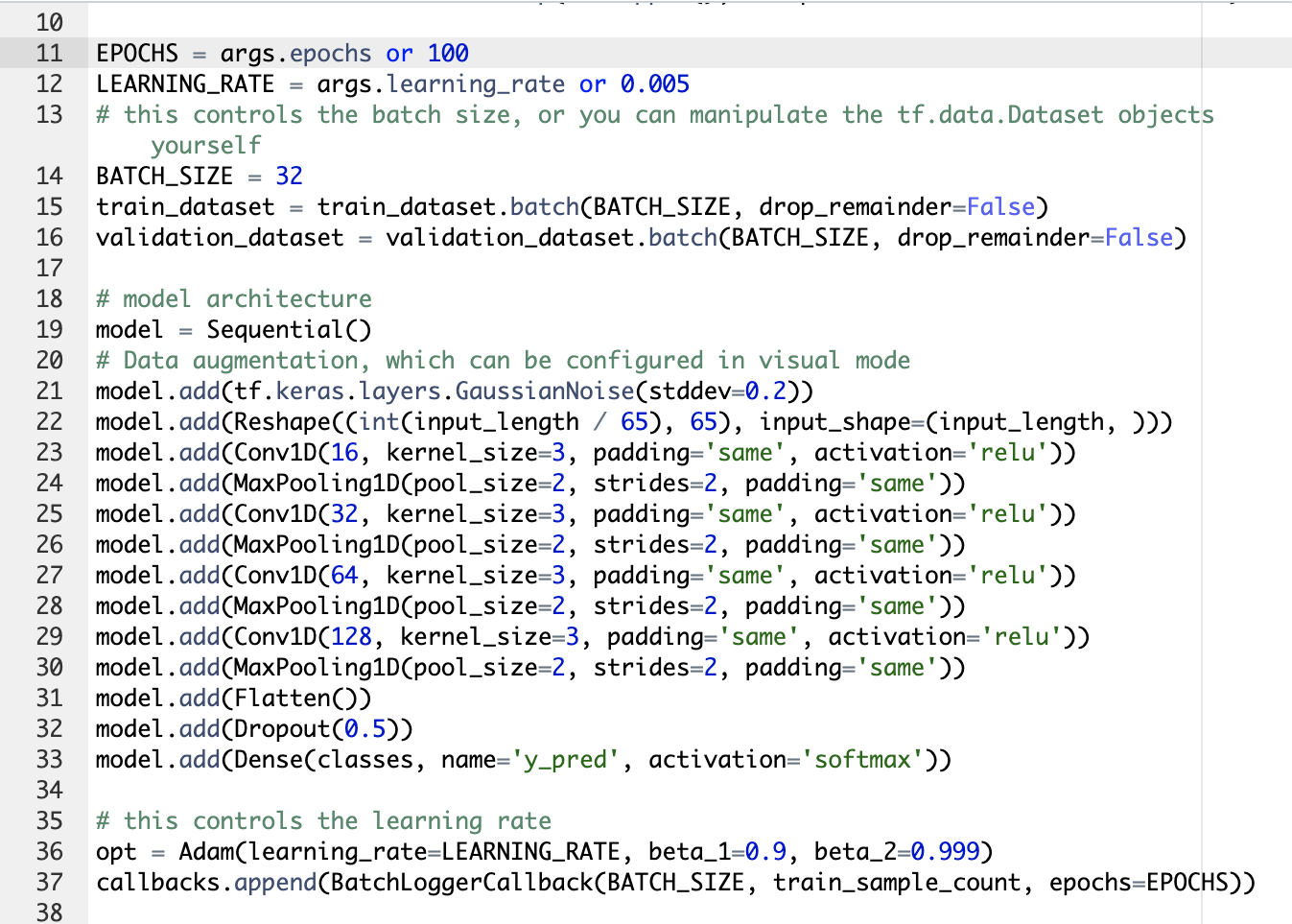
|
Figure 8. Model architecture
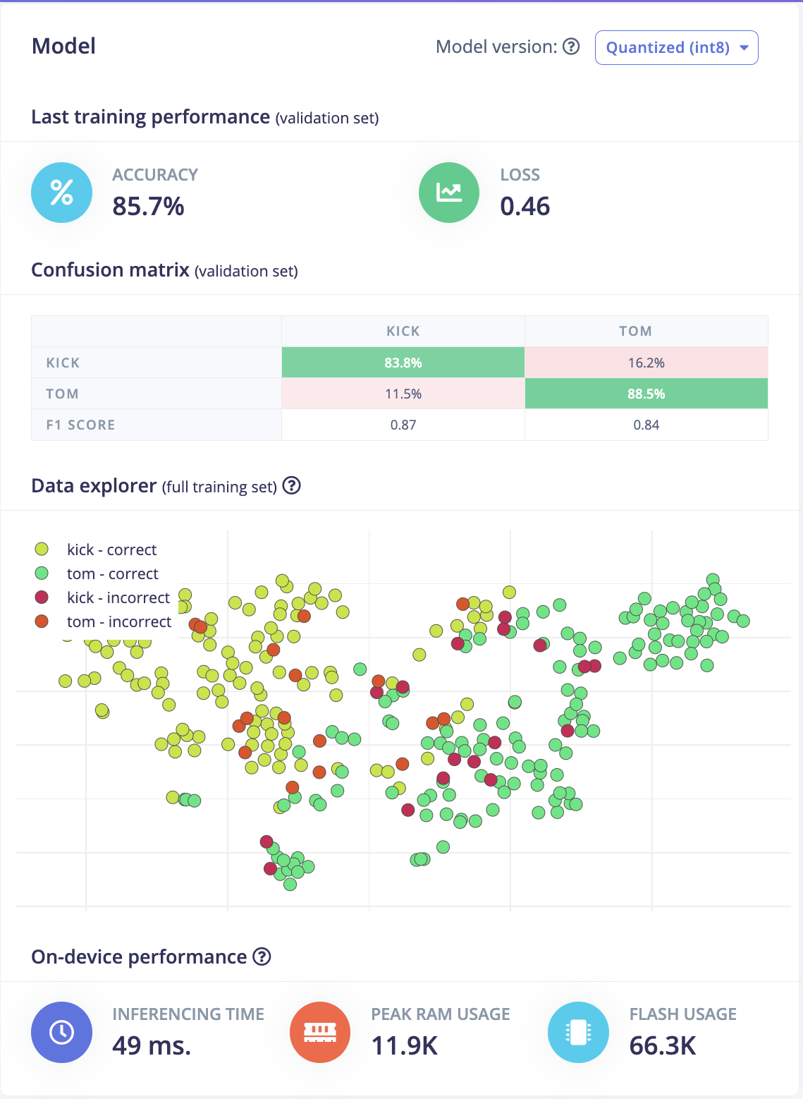
Lastly, the deployment of the model on an Arduino have produced a report for peak RAM usage of 11.9kb and a flash usages of 66.3kb were found to be moderate, indicating that the model was relatively lightweight and suitable for such kind of sensor (with 1MB flash and 256kb SRAM).
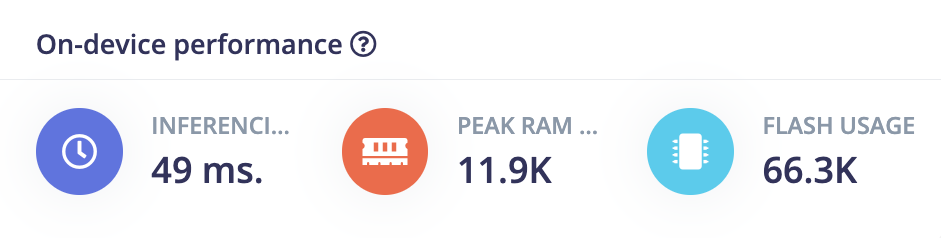
Figure 9. Report of on device performance
The project has explored different models with combinations of parameters. There are mainly 3 models suitable for audio processing on Edge Impulse: MFE, MFCC and Spectrogram. These models mainly differentiates in data preprocessing. All models takes the approach of windowing and fourier transformation so that the continuous signal are clipped into smaller segments with smooth edges. The MFE model further puts a filter over signal collected to imitate the human hearing ability. Based on this filter, the MFCC model extracts information in a higher dimension (contains more features) by considering the shape of the spectrum (more detailed information please refer to appendix[iii]). A illustration of the differences of the 3 models is shown as follows.
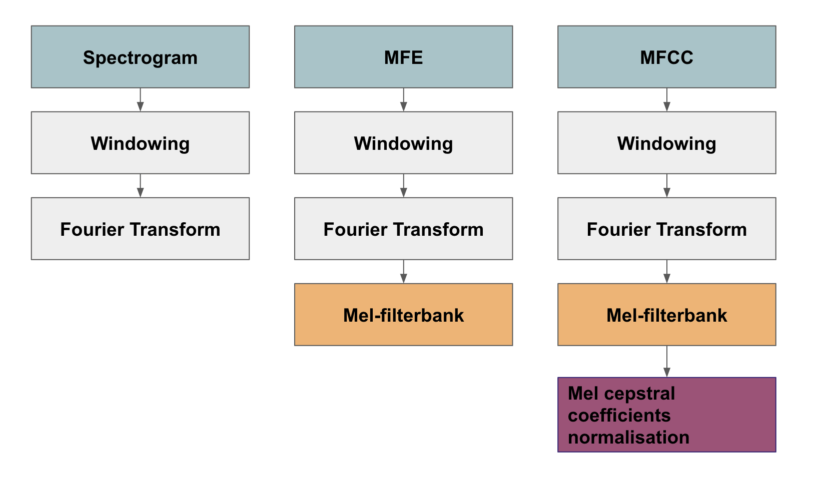
Figure 9. Data preprocessing in Spectrogram, MFE and MFCC models
The data collected was first fitted with auto-tuned Raw-feature, Spectrogram, MFE and MFCC models. It can be noticed that, a raw-data model has given the worst accuracy of 60.3% in validation and 53.73% in test data by putting the raw frequency of audio signal into a neural network with 2 layers (less training cycles here is used to prevent overfit and under performance on test data). By incorporating the technique of slicing up the continuous frequency into windows, making spectrogram by Fourier transform and stacking them up (the preprocessing blocks shared by Spectrogram, MFE and MFCC), the performance of the models has improved by over 16% on validation set and 10% on test set.
| model | training cycles | learning rate | validation score | test score |
|---|---|---|---|---|
| raw-data | 30 | 0.05 | 60% | 54% |
| spectrogram | 100 | 0.005 | 76% | 64% |
| MFE | 100 | 0.005 | 79% | 76% |
| MFCC | 100 | 0.005 | 78% | 70% |
Table 1: Comparison between 4 prefitted models.
Knowing that the windowing and Fourier transformation could greatly improve the model performance, the project has turned to transfer learning using the EON model pre-trained by Edge Impulse. By converting the raw signal collected to spectrograms via Fourier transformation, the resulting images can be analyzed for patterns using this large image classification model, which may leverage the strengths of both the Fourier transformation and the pre-trained EON model to better distinguish between different types of sounds. The EON tuning tool identified a version of spectrogram models 'spectr-conv1d-6df' as the optimal choice with best performance on validation scores. However, the latency of the optimal model has exceeded the tuning target by 5389ms per inference even though it has the best accuracy scores. This version of Spectrogram model was used to update the previous blocks in my project and its parameters 'frames length', 'frame stride' and 'FFT length' are changed to investigate if better accuracy can be achieved. The results are logged in tables2. As can be seen in the table, the optimal window size (frame length) is 0.025 seconds. The comparisons between cases 1 and 2, 4 and 5 indicate that Overlappings between 2 neighbouring windows does not help in producing better results. 2 to 3 times peak RAM usage can be generated if 256 data point sampled in one frequency cycle compared to the cases where 128 are sampled. In addition, FFT length of 256 gives a better resolution but may cause overfitting in training data as can be observed in case pairs 3 and 8, 4 and 8, where validation score improved by 1.6% and test score remain unchanged. The parameters in case 1 were adopted eventually.
| index | Frame Length | Frame Stride | FFT length | validation score | test score | peak RAM | Flash Usage |
|---|---|---|---|---|---|---|---|
| 1 | 0.025 | 0.025 | 128 | 85.7% | 82.9% | 11.9k | 66.3k |
| 2 | 0.025 | 0.01 | 128 | 76.2% | 71.64% | 12.6k | 69.1k |
| 3 | 0.01 | 0.01 | 128 | 79.4% | 79.1% | 19.5k | 67.3k |
| 4 | 0.05 | 0.05 | 128 | 71.4% | 76.12% | 9.4k | 66.1k |
| 5 | 0.05 | 0.025 | 128 | 76.2% | 67.16% | 11.8k | 66.3k |
| 6 | 0.025 | 0.025 | 256 | 77.8% | 82.09% | 17.7k | 69.3k |
| 7 | 0.01 | 0.01 | 256 | 81.0% | 79.1% | 32.8k | 70.3k |
| 8 | 0.05 | 0.05 | 256 | 76.2% | 76.12% | 12.6k | 69.1k |
Table 2: Tuning Frame Length and Frame Stride.
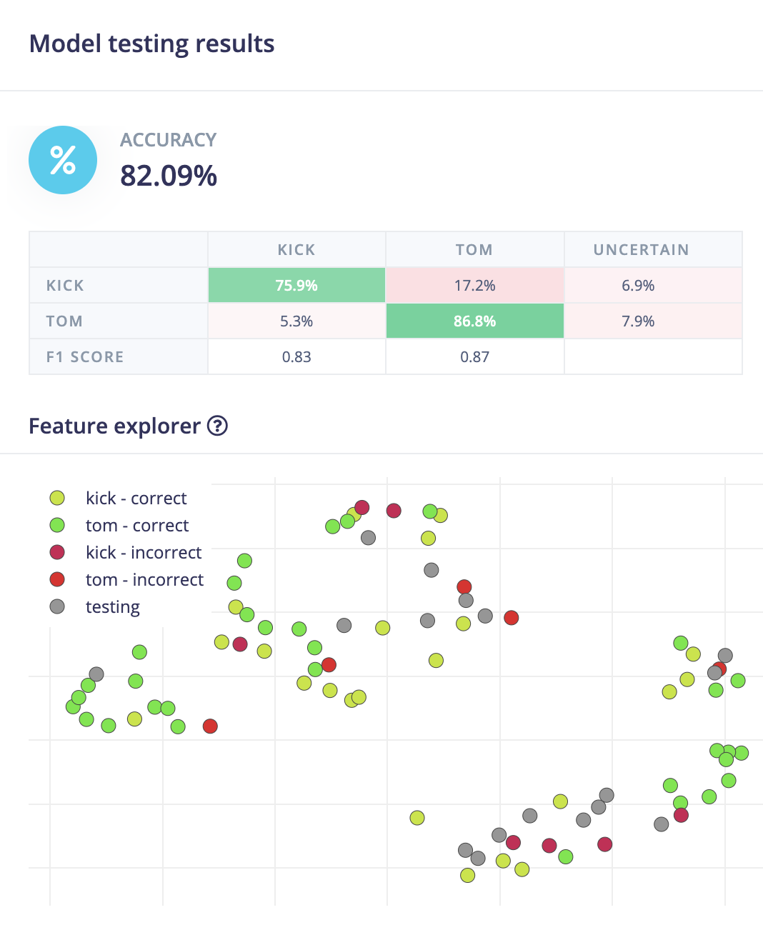
the results of the model selected are shown below. Spectr-conv1d-6df has produced an accuracy of 85.7% on validation set and 82.09% on test set. The results may indicate a relative high reliability of the model in classifying sound clips engineered for 'kicks' and 'toms'.
|
|
Figure 10: Model results on validation set and test set.
The demo task focused on exploring how to extract features from different sound clips theoretically, to develop an application that can distinguish based on these features. Data was sampled using an audio loopback driver called 'Blackhole', which records directly from the computer's audio interface to minimize noise. Time series without data (where no oscillation is seen in the frequency graph) were then removed from the recorded clips. However, this model may not perform well in the final project due to three main reasons: 1. It does not consider background noise and signal loss during transmission when the model is deployed on a sensor. 2. Collecting background noise (either from the environment or by looping back audio data) to imitate the real-world scenario of a sensor collecting data would require additional workload; 3. The data amount (1m17s) was relatively insufficient.
In the final project, audio clips are recorded directly by the Arduino sensor with background noise, which can be beneficial for several reasons: 1. It accounts for signal loss during transmission through air, allowing the model to focus on distinguishing different instruments; 2. it uses the same sensor to collect data directly on which the model will later be deployed, potentially leading to better performance; 3. By keeping the time span with pure noise before the instrument comes in, the model can better capture the attack of the sound and may extract valuable features; 4. the data amount has increased from 1m17s to 10m10s.
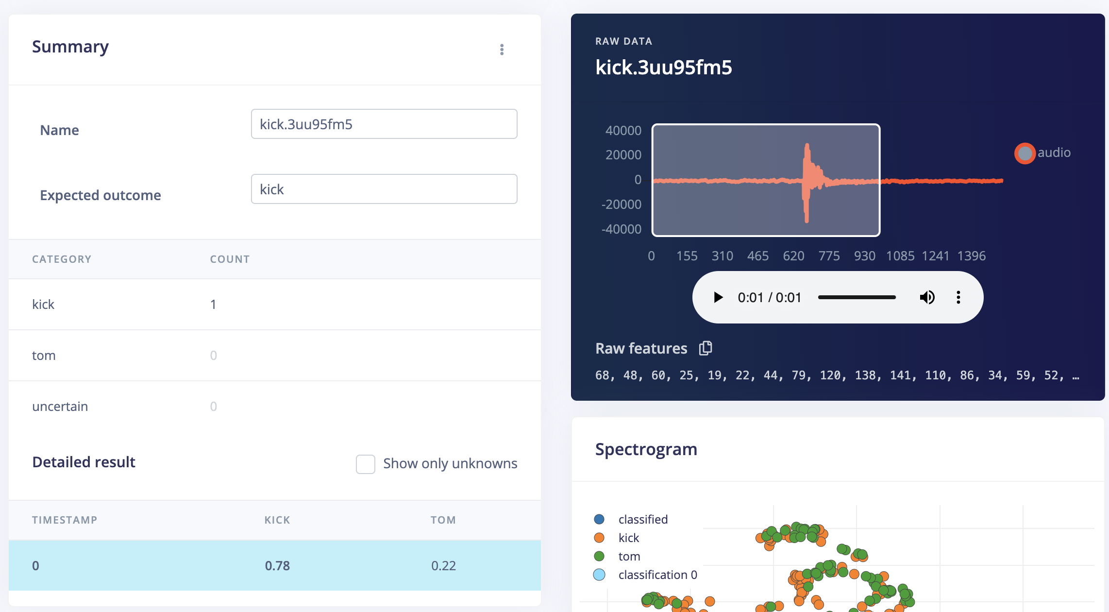
The model was broadly tested by a wide range of sound clips labelled toms and kicks. And these test samples are also characterized in their names as 'cinematic', 'acoustic' etc, which may indicate these clips are quite different in design even within each label. Utilizing the variety of clips can be It was noticed that the difference in resonation and change in frequencies of the two types of sounds are well captured by the model. The figure below shows, a kick that appears to have longer resonation (can be engineered by managing decay and release, please refer to appendix[iii] for detailed information) was misclassified as tom, and vice versa, a tom that has shorter resonation and sooner attack can be misclassified as kick.
|
|
Figure 11: An example of false classification (kick with longer resonation) on the right, compared to a typical kick with short resonation and louder attack on the left.
Moreover, although spectrogram models do not perform as well as MFE or MFCC models during the pre-fitting stage, they seem to outperform the latter two after fine-tuning. This suggests that for instrumental sound clip classification tasks that transfer raw frequencies to spectrograms, deep learning models may perform better without reducing the higher frequency range or mimicking human perception. Additionally, incorporating cepstral coefficients may not be necessary and may overfit the training set by adding an extra dimension for such tasks that only focus on the tone colors of sounds (see table 1).
If I had more time to work on this project, it could be further developed in the following ways:
- Adding more types of instruments to the collection.
- Incorporating more variations in tone for each instrument.
- Taking into consideration the factor of sound field. The position of different instruments has general guidelines and conventions, and often be engineered in electronic music production. This aspect may help us classify the instrument from its sound clip as an additional reference.
- Increase the amount of data to be trained.
-
- the project on edge impulse: https://studio.edgeimpulse.com/public/217672/latest
-
- the demo project on edge impulse: https://studio.edgeimpulse.com/public/199755/latest
-
- Demo task presentation1: https://www.youtube.com/watch?v=_bu1VxgMrQs&t=562s
-
- Demo task presentation2: https://www.youtube.com/watch?v=WKzNbHNQhQc&t=323s
- Arduino Library (no date) Arduino library - Edge Impulse Documentation. Available at: https://docs.edgeimpulse.com/docs/deployment/arduino-library (Accessed: April 29, 2023).
- Arduino nano 33 ble sense (no date) Arduino Nano 33 BLE Sense - Edge Impulse Documentation. Available at: https://docs.edgeimpulse.com/docs/development-platforms/officially-supported-mcu-targets/arduino-nano-33-ble-sense (Accessed: April 29, 2023).
- Arduino nano 33 ble sense REV2 (no date) Arduino Official Store. Available at: https://store.arduino.cc/products/nano-33-ble-sense-rev2?gclid=Cj0KCQjwgLOiBhC7ARIsAIeetVBhlAOKVwvvmz9SACyagg8Fqprz_yf8vFp8xQK5vKkbtoibmFFnEuwaAjjUEALw_wcB (Accessed: April 29, 2023).
- Eon Tuner (no date) EON Tuner - Edge Impulse Documentation. Available at: https://docs.edgeimpulse.com/docs/edge-impulse-studio/eon-tuner (Accessed: April 29, 2023).
- Recognize sounds from audio (no date) Recognize sounds from audio - Edge Impulse Documentation. Available at: https://docs.edgeimpulse.com/docs/tutorials/audio-classification (Accessed: April 29, 2023).
- Splice sample packs (no date) Splice. Available at: https://splice.com/sounds/labels/splice (Accessed: April 29, 2023).
I, Borui Wei, confirm that the work presented in this assessment is my own. Where information has been derived from other sources, I confirm that this has been indicated in the work
Borui Wei, 27/04/2023