Data structures and Algorithms

Complexity (Big O)

Complexity of an algorithm measures time and memory. How long does one algorithm takes to finish? How much memory does it use?

We measure these values in terms of the input size (Usually for the input size we use the letter $n$)

We can analyze algorithms in the Best case, Average case and Worst case.

Best case measures the quickest way for an algorithm to finish.

Average case measures what time does the algorithm need to finish on average.

Worst case measures the slowest time for an algorithm to finish.

General idea

1. Big O: - the algorithm takes at most steps to finish in the WORST CASE.
2. Little o: - the algorithm takes less than steps to finish in the WORST CASE.
3. Big Omega: - the algorithm takes at least steps to finish in the BEST CASE.
4. Little Omega: - the algorithm takes more than steps to finish in the BEST CASE.
5. Big Theta: - the combination of and . Meaning the algorithm takes at least steps to finish and takes at most steps to finish, i.e. it always takes steps.

Comparison of orders of common functions

Big O cheat sheet

https://www.bigocheatsheet.com/

Formal definitions

Examples

means that if our algorithm takes input of 10 elements it will need 100 steps to finish in the worst case. If the input is of 100 elements it will need 10000 steps to finish in the worst case.

Constants and Big O

Usually we discard constants when using Big O, but in some cases the constant can be meaningful for small input sizes. In the following example is faster than because our complexities are and so for the algorithm is faster than the one.

Sorting

Sorting means ordering a set of elements in a sequence.

We can sort a set of elements whose elements are in partial order. Partial order is a relation with the following properties:

1. Antisymmetry - For every 2 elements in the set (A, B), if and then .
2. Transitivity - For every 3 elements in the set (A, B, C), if and then .
3. Reflexivity - For every element in the set A, .

Sorting properties

Stable sort

A sorting algorithm is stable if two equal objects appear in the same order in the ordered output as they appeared in the unsorted input.

Example input: . Here and are simply a 3 but we have marked them to follow what happens with them after the sorting.

Example output:

Unstable sort output:

In place sort

Uses only a small constant amount of extra memory. In place sort means the elements are swapped around. Out of place means we use another extra array to swap items around.

Number of comparisons

How many times do we need to compare 2 elements. For most sorts this represents the time complexity.

Adaptive sort

Determines whether the sorting algorithm runs faster for inputs that are partially or fully sorted. If an algorithm is unadaptive it runs for the same time on sorted and unsorted input. If an algorithm is adaptive it runs faster on sorted input than on unsorted input.

Online sort

Determines if an algorithm needs all the items from the input to start sorting. If an algorithm is online it can start sorting input that is given in parts. If an algorithm is offline it can start sorting only after it has the whole input.

External sort

Allows sorting data which cannot fit into memory. Such algorithms are designed to sort massive amounts of data (Gigabytes, Terabytes, etc.)

Parallel sort

An algorithm which can be ran on multiple threads at the same time, speeding the running time.

Locality

An algorithm which heavily uses the processor cache to speed up its execution. The data processed needs to be sequentially located.

Helper code

// swap the values of two variables
void swap(int & a, int & b) {
    int tmp = a;
    a = b;
    b = tmp;
}

Bubble sort

Bubble sort	n = input size
Time complexity
Space complexity
Adaptive	Yes
Stable	Yes
Number of comparisons
Number of swaps
Online	No
In place	Yes

Honorable mention - Cocktail shaker sort, similar to bubble and selection sort. It’s like the Online version of bubble sort.

Clean code

void bubbleSort(int * array, int length) {
    for (int bubbleStartIndex = 0; bubbleStartIndex < length; bubbleStartIndex++) {
        for (int bubbleMovedIndex = 0; bubbleMovedIndex < length - 1; bubbleMovedIndex++) {
            if (array[bubbleMovedIndex] > array[bubbleMovedIndex+1]) {
                swap(array[bubbleMovedIndex], array[bubbleMovedIndex+1]);
            }
        }
    }
}

Short code

void bubbleSort(int * array, int length) {
    for (int i = 0; i < length; i++) {
        for (int k = 0; k < length - 1; k++) {
            if (array[k] > array[k+1]) {
                swap(array[k], array[k+1]);
            }
        }
    }
}

Optimization 1 - make it faster

void bubbleSort(int * array, int length) {
    for (int i = 0; i < length; i++) {
        for (int k = 0; k < length - 1 - i; k++) { // length - 1 - i = 2x less iterations
            if (array[k] > array[k+1]) {
                swap(array[k], array[k+1]);
            }
        }
    }
}

Optimization 2 - make it adaptive

void bubbleSort(int * array, int length) {
    for (int i = 0; i < length; i++) {
        bool swappedAtLeastOnce = false; // add a flag to check if a swap has occurred

        for (int k = 0; k < length - 1 - i; k++) {
            if (array[k] > array[k+1]) {
                swap(array[k], array[k+1]);
                swappedAtLeastOnce = true;
            }
        }
        
        if (!swappedAtLeastOnce) { // if there were no swaps, it's ordered
            break;
        }
    }
}

Selection sort

Selection sort	n = input size
Time complexity
Space complexity
Adaptive	No
Stable	No
Number of comparisons
Number of swaps
Online	No
In place	Yes

Key points

1. It’s better than bubble sort in cases we need to sort items which are very large in size because it has $\mathcal{O}(n)$ swaps.

Clean code

void selectionSort(int * array, int length) {
    for (int currentIndex = 0; currentIndex < length; currentIndex++) {
        int smallestNumberIndex = currentIndex;

        for (int potentialSmallerNumberIndex = currentIndex + 1; 
             	potentialSmallerNumberIndex < length;
             	potentialSmallerNumberIndex++) {
            if (array[potentialSmallerNumberIndex] < array[smallestNumberIndex]) {
                smallestNumberIndex = potentialSmallerNumberIndex;
            }
        }
        
        swap(array[currentIndex], array[smallestNumberIndex]);
    }
}

Short code

void selectionSort(int * array, int length) {
    for (int i = 0; i < length; i++) {
        int index = i;

        for (int k = i + 1; k < length; k++) {
            if (array[k] < array[index]) {
                index = k;
            }
        }
        
        swap(array[i], array[index]);
    }
}

Insertion sort

Insertion sort	n = input size
Time complexity
Space complexity
Adaptive	Yes
Stable	Yes
Number of comparisons
Number of swaps
Online	Yes
In place	Yes

Key points

1. The best algorithm for sorting small arrays.
2. Often combined with other algorithms for optimal runtime.

Clean code

void insertionSort(int * array, int length) {
    for (int nextItemToSortIndex = 1; nextItemToSortIndex < length; nextItemToSortIndex++) {
        for (int potentiallyBiggerItemIndex = nextItemToSortIndex; 
             	potentiallyBiggerItemIndex > 0 && 
             	array[potentiallyBiggerItemIndex] < array[potentiallyBiggerItemIndex - 1];
             	potentiallyBiggerItemIndex--) {
            swap(array[potentiallyBiggerItemIndex], array[potentiallyBiggerItemIndex-1]);
        }
    }
}

Short code

void insertionSort(int * array, int length) {
    for (int i = 1; i < length; i++) {
        for (int k = i; k > 0 && array[k] < array[k - 1]; k--) {
            swap(array[k], array[k-1]);
        }
    }
}

Merge sort

Merge sort	n = input size
Time complexity
Space complexity
Adaptive	No
Stable	Yes
Number of comparisons
External	Yes
Parallel	Yes
Online	No
In place	No

Key points

1. Every array of 0 or 1 elements is sorted.
2. Merging requires additional memory.
3. Splitting the array in 2 every time gives us $log(n)$ levels.
4. On each level we have $\mathcal{O}(n)$ for the merging operation.

Honorable mention - Ford–Johnson aka. Merge-insertion sort. Cool idea, but not practical enough.

Important algorithm: Timsort - Absolute beast with worst case and best case. Implementation can be found here: https://github.com/tvanslyke/timsort-cpp

Clean code

void merge(int * originalArray, int * mergeArray, int start, int mid, int end) {
    int leftIndex = start;
    int rightIndex = mid + 1;
    int sortedIndex = start;

    while (leftIndex <= mid && rightIndex <= end) {
        if (originalArray[leftIndex] <= originalArray[rightIndex]) {
            mergeArray[sortedIndex] = originalArray[leftIndex];
            leftIndex++;
        } else {
            mergeArray[sortedIndex] = originalArray[rightIndex];
            rightIndex++;
        }

        sortedIndex++;
    }

    while (leftIndex <= mid) {
        mergeArray[sortedIndex] = originalArray[leftIndex];
        leftIndex++;
        sortedIndex++;
    }
    while (rightIndex <= end) {
        mergeArray[sortedIndex] = originalArray[rightIndex];
        rightIndex++;
        sortedIndex++;
    }

    for (int i = start; i <= end; i++) {
        originalArray[i] = mergeArray[i];
    }
}

void mergeSortRecursive(int * original, int * mergeArray, int start, int end) {
    if (start < end) {
        int mid = (start + end) / 2;

        mergeSortRecursive(original, mergeArray, start, mid);
        mergeSortRecursive(original, mergeArray, mid + 1, end);

        merge(original, mergeArray, start, mid, end);
    }
}

void mergeSort(int * array, int length) {
    int * mergeArray = new int[length];
    mergeSortRecursive(array, mergeArray, 0, length - 1);
    delete[] mergeArray;
}

Short code

void merge(int * originalArray, int * mergeArray, int start, int mid, int end) {
    int left = start;
    int right = mid + 1;

    for (int i = start; i <= end; i++) {
        if (left <= mid && (right > end || originalArray[left] <= originalArray[right])) {
            mergeArray[i] = originalArray[left];
            left++;
        } else {
            mergeArray[i] = originalArray[right];
            right++;
        }
    }

    for (int i = start; i <= end; i++) {
        originalArray[i] = mergeArray[i];
    }
}

void mergeSortRecursive(int * originalArray, int * mergeArray, int start, int end) {
    if (start < end) {
        int mid = (start + end) / 2;

        mergeSortRecursive(originalArray, mergeArray, start, mid);
        mergeSortRecursive(originalArray, mergeArray, mid + 1, end);

        merge(originalArray, mergeArray, start, mid, end);
    }
}

void mergeSort(int * array, int length) {
    int * mergeArray = new int[length];
    mergeSortRecursive(array, mergeArray, 0, length - 1);
    delete[] mergeArray;
}

Quick sort

Quick sort	n = input size
Time complexity (Worst case)
Time complexity (Average case)
Space complexity
Adaptive	No
Anti-Adaptive	Yes (the more randomness, the better)
Stable	No
Number of comparisons
Parallel	Yes
Online	No
In place	Yes
Locality	Yes

Key points

1. Quick sort adores chaos. That’s why a common strategy is to shuffle the array before sorting it.

C++ STL sorting algorithm is Introsort, which is a hybrid between quicksort and heapsort.

Quick sort optimization for arrays with many equal numbers - three-way partitioning, aka Dutch national flag.

Quick sort can also be optimized with picking 2 pivots instead of 1 - multi-pivot quicksort.

Why is quick sort usually faster than merge sort and other fast algorithms?

The table bellow is an approximation of the time required to access data from the disk/ram/CPU cache. It gives us an idea why quick sort is indeed quick. Quick sort being in-place gets reduced to problems in the CPU cache very fast. Merge sort on the other hand uses additional memory, so it has 2 arrays it works with essentially. Often these 2 arrays cannot simultaneously enter the cache so they have to be read from RAM, which is very slow. Quick sort, however, uses only one array which gets pulled into the CPU cache and operations on it are very fast.

Memory hierarchy	CPU cycles	size
HDD	500, 000	1 TB
RAM	100	4 GB
L2 cache	10	512 kb
L1 cache	1	32 kb

Uses apart from sorting

1. Find k-th biggest/smallest element

Clean code using Lomuto partitioning

int partition(int * array, int startIndex, int endIndex) {
    int pivot = array[endIndex];
    int pivotIndex = startIndex;

    for (int i = startIndex; i <= endIndex; i++) {
        if (array[i] < pivot) {
            swap(array[i], array[pivotIndex]);
            pivotIndex++;
        }
    }

    swap(array[endIndex], array[pivotIndex]);
    return pivotIndex;
}

void _quickSort(int * array, int startIndex, int endIndex) {
    if (startIndex < endIndex) {
        int pivot = partition(array, startIndex, endIndex);
        _quickSort(array, startIndex, pivot - 1);
        _quickSort(array, pivot + 1, endIndex);
    }
}

void quickSort(int * array, int length) {
    _quickSort(array, 0, length - 1);
}

Short code using Lomuto partitioning

int partition(int * array, int start, int end) {
    int pivot = array[end];
    int pivotIndex = start;
    for (int i = start; i <= end; i++) {
        if (array[i] < pivot) {
            swap(array[i], array[pivotIndex]);
            pivotIndex++;
        }
    }
    swap(array[end], array[pivotIndex]);
    return pivotIndex;
}

void _quickSort(int * array, int start, int end) {
    if (start < end) {
        int pivot = partition(array, start, end);
        _quickSort(array, start, pivot - 1);
        _quickSort(array, pivot + 1, end);
    }
}

void quickSort(int * array, int length) {
    _quickSort(array, 0, length - 1);
}

Optimization 1 - pivot is random number

#include <random>
int generateRandomNumber(int from, int to) {
    std::random_device dev;
    std::mt19937 rng(dev());
    std::uniform_int_distribution<std::mt19937::result_type> dist6(from,to);

    return dist6(rng);
}

int partition(int * array, int start, int end) {
    int randomIndex = generateRandomNumber(start, end);
    swap(array[end], array[randomIndex]);
    
    int pivot = array[end];
    int pivotIndex = start;
    for (int i = start; i <= end; i++) {
        if (array[i] < pivot) {
            swap(array[i], array[pivotIndex]);
            pivotIndex++;
        }
    }
    swap(array[end], array[pivotIndex]);
    return pivotIndex;
}

void _quickSort(int * array, int start, int end) {
    if (start < end) {
        int pivot = partition(array, start, end);
        _quickSort(array, start, pivot - 1);
        _quickSort(array, pivot + 1, end);
    }
}

void quickSort(int * array, int length) {
    _quickSort(array, 0, length - 1);
}

Optimization 2 - shuffle before picking pivot

#include <random>
int generateRandomNumber(int from, int to) {
    std::random_device dev;
    std::mt19937 rng(dev());
    std::uniform_int_distribution<std::mt19937::result_type> dist6(from,to);

    return dist6(rng);
}

void shuffle(int * arr, int length) {
    for (int i = 0; i < length - 1; i++) {
        int swapCurrentWith = generateRandomNumber(i, length - 1);
        swap(arr[i], arr[swapCurrentWith]);
    }
}

int partition(int * array, int start, int end) {
    shuffle(array + start, end - start);

    int pivot = array[end];
    int pivotIndex = start;
    for (int i = start; i <= end; i++) {
        if (array[i] < pivot) {
            swap(array[i], array[pivotIndex]);
            pivotIndex++;
        }
    }
    swap(array[end], array[pivotIndex]);
    return pivotIndex;
}

void _quickSort(int * array, int start, int end) {
    if (start < end) {
        int pivot = partition(array, start, end);
        _quickSort(array, start, pivot - 1);
        _quickSort(array, pivot + 1, end);
    }
}

void quickSort(int * array, int length) {
    _quickSort(array, 0, length - 1);
}

Short code using Hoare partitioning

int partition(int * array, int start, int end)  {
    int pivot = array[(start + end) / 2];
    int left = start - 1;
    int right = end + 1;

    while (true) {
        do {
            left++;
        } while (array[left] < pivot);

        do {
            right--;
        } while (array[right] > pivot);

        if (left >= right) {
            return right;
        }

        swap(array[left], array[right]);
    }
}

void _quickSort(int * array, int start, int end) {
    if (start < end) {
        int pivot = partition(array, start, end);
        _quickSort(array, start, pivot - 1);
        _quickSort(array, pivot + 1, end);
    }
}

void quickSort(int * array, int length) {
    _quickSort(array, 0, length - 1);
}

Counting sort

Counting sort	n = input size, k = max number
Time complexity (Worst case)
Time complexity (Best case)
Space complexity

Key points

1. Not a comparison sort.
2. Very efficient for an array of integers with many repeating integers with small difference between the biggest and smallest integer.

Uses apart from sorting

1. Counting inversions

Counting sort for positive numbers

void countingSort(int * array, int length) {
    int maxNumber = 0;
    for (int i = 0; i < length; i++) {
        if (array[i] > maxNumber) {
            maxNumber = array[i];
        }
    }

    int * countingArray = new int[maxNumber + 1];
    for (int i = 0; i < maxNumber + 1; i++) {
        countingArray[i] = 0;
    }

    for (int i = 0; i < length; i++) {
        countingArray[array[i]]++;
    }

    int sortedIndex = 0;
    for (int i = 0; i < length; i++) {
        while (countingArray[sortedIndex] == 0) {
            sortedIndex++;
        }

        array[i] = sortedIndex;
        countingArray[sortedIndex]--;
    }

    delete[] countingArray;
}

Bucket sort

Bucket sort	n = input size, k = number of buckets
Time complexity (Worst case)
Time complexity (Average case)
Space complexity

Key points

1. It’s a distribution sort, not a comparison sort.
2. Very situational sort.
3. The bellow code is a sample implementation for floats between 0 and 1.

Code

#include <iostream>
#include <vector>
#include <algorithm>
void bucketSort(double *array, int length) {
    std::vector<double> buckets[length];

    for(int i = 0; i < length; i++) {
        buckets[int(length * array[i])].push_back(array[i]);
    }

    for(int i = 0; i < length; i++) {
        sort(buckets[i].begin(), buckets[i].end());
    }

    int index = 0;
    for(int i = 0; i < length; i++) {
        while(!buckets[i].empty()) {
            array[index] = buckets[i][0];
            index++;
            buckets[i].erase(buckets[i].begin());
        }
    }
}

Radix sort

Radix sort

Radix sort	n = input size
Time complexity (Worst case)
Time complexity (Average case)
Space complexity

Key points

1. Good on multi-threaded machines.

Code

#include <iostream>
#include <cmath>
#include <list>

int abs(int a) {
    return a >= 0 ? a : -a;
}

void radixSort(int * array, int length) {
    int maxNumber = 0;
    for (int i = 0; i < length; i++) {
        if (abs(array[i]) > maxNumber) {
            maxNumber = abs(array[i]);
        }
    }

    int maxDigits = log10(maxNumber) + 1;

    std::list<int> pocket[10];

    for(int i = 0; i < maxDigits; i++) {
        int m = pow(10, i + 1);
        int p = pow(10, i);

        for(int j = 0; j < length; j++) {
            int temp = array[j] % m;
            int index = temp / p;
            pocket[index].push_back(array[j]);
        }

        int count = 0;
        for(int j = 0; j<10; j++) {
            while(!pocket[j].empty()) {
                array[count] = *(pocket[j].begin());
                pocket[j].erase(pocket[j].begin());
                count++;
            }
        }
    }
}

Searching

Linear search

Linear search	n = input size
Time complexity
Space complexity

Algorithm idea

Iterate every element in order and check if it is the element we are looking for.

Code

int linearSearch(int *array, int length, int target) {
    for (int i = 0; i < length; i++) {
        if (array[i] == target) {
            return i;
        }
    }
    return -1;
}

Uses

Searching in unordered data, when we have very few queries. If we have many queries it’s better to sort the array and use faster searching for the queries.

Binary search

Binary search	n = input size
Time complexity
Space complexity

Works only on sorted array-like structures, which support $\mathcal{O}(1)$ access to elements.

The algorithm uses $\mathcal{O}(log(n))$ space if written recursively, but can be written iteratively to have $\mathcal{O}(1)$ space as well.

Algorithm idea

1. Check the middle element, if it’s the element we are looking for - we are done
2. If the element is bigger than the one we are looking for - recurse into the left sub-array (the sub-array with smaller elements).
3. If the element is smaller than the one we are looking for - recurse into the right sub-array (the sub-array with bigger elements).

Code

int binarySearch(int *array, int length, int target) {
    int left = 0;
    int right = length - 1;

    while(left <= right) {
        int mid = (left + right) / 2;

        if (array[mid] == target) {
            return mid;
        }
        if (array[mid] > target) {
            right = mid - 1;
        }
        if (array[mid] < target) {
            left = mid + 1;
        }
    }

    return -1;
}

Uses

Fast searching in ordered data.

Guess and check algorithms.

Ternary search

Ternary search	n = input size
Time complexity
Space complexity

Algorithm idea

The same idea as binary search but we split the array in 3 parts. On each step we decide which one part to discard and recurse into the other 2.

Code

int ternarySearch(int *array, int length, int target) {
    int left = 0;
    int right = length - 1;

    while (left <= right) {
        int leftThird = left + (right - left) / 3;
        int rightThird = right - (right - left) / 3;

        if (array[leftThird] == target) {
            return leftThird;
        }
        if (array[rightThird] == target) {
            return rightThird;
        }

        if (target < array[leftThird]) {
            right = leftThird - 1;
        } else if (target > array[rightThird]) {
            left = rightThird + 1;
        } else  {
            left = leftThird + 1;
            right = rightThird - 1;
        }
    }

    return -1;
}

Uses

Finding min/max in a sorted array.

Exponential search

Exponential search	n = input size
Time complexity
Space complexity

Algorithm idea

This is the binary search algorithm applied for ordered data of unknown size. We don’t have a mid point so we start from the beginning and double our guessed index each time. e.g for guessed index: 1, 2, 4, 8, 16, 32... If we overshoot the end of the data we go back using binary search because we now have an end index. e.g for array with 27 elements we do a jump to element 32 which doesn’t exist and then use binary search on elements 16 - 32.

Code

int exponentialSearch(int *array, int length, int target) {
   if (length == 0) {
      return false;
   }

   int right = 1;
   while (right < length && array[right] < target) {
      right *= 2;
   }

   int binaryIndex = binarySearch(array + right/2, min(right + 1, length) - right/2, target);
   if (binaryIndex != -1) {
      return binaryIndex + right/2;
   } else {
      return -1;
   }
}

Uses

Binary search on streams, which are ordered and other ordered data of unknown size.

Jump search

Jump search	n = input size
Time complexity
Space complexity

Algorithm idea

We decide on a jump step and check elements on each step. e.g for step 32 we will check elements 0, 32, 64, etc.

Optimal jump step is $\sqrt{n}$.

Code

int jumpSearch(int *array, int length, int target) {
   int left = 0;
   int step = sqrt(length);
   int right = step;

   while(right < length && array[right] <= target) {
      left += step;
      right += step;
      if(right > length - 1)
         right = length;
   }

   for(int i = left; i < right; i++) {
      if(array[i] == target)
         return i;
   }

   return -1;
}

Uses

Because it’s worse than Binary search, it’s useful when the data structure we are searching in has very slow jump back, aka it’s slow to go back to index $i - 10$ from $i$.

Interpolation search

Interpolation search	n = input size
Time complexity for evenly distributed data
Time complexity for badly distributed data
Space complexity

Algorithm idea

If we have well distributed data we can approximate where we will find the element with the following formula Example for well distributed data: 1, 2, 3, 4, 5, 6 .... 99, 100

Example for badly distributed data: 1, 1, 1, 1.... 1, 1, 100

Code

int interpolationSearch(int *array, int length, int target) {
    int left = 0;
    int right = length - 1;

    while (array[right] != array[left] && target >= array[left] && target <= array[right]) {
        int mid = left + ((target - array[left]) * (right - left) / (array[right] - array[left]));

        if (array[mid] < target)
            left = mid + 1;
        else if (target < array[mid])
            right = mid - 1;
        else
            return mid;
    }

    if (target == array[left])
        return left;
    else
        return -1;
}

Uses

Very situational, when we have data which is evenly distributed.

Linked lists

Linked list stores its data in separate Nodes. Each node points the next node in the list. The last node points NULL.

The most primitive linked list’s node contains 2 fields - Data and Next pointer

struct Node {
	int data;
	Node* next;
};

Complexity comparison

Operation / Data structure	Array	Singly linked list without tail	Singly linked list with tail	Doubly linked list without tail	Doubly linked list with tail
push_front
pop_front
get_front
push_back
pop_back
get_back
get_at
find_key
erase_key
is_empty
add_before
add_after

Memory allocation

Array

Linked list

Use

Linked lists are useful if we don’t know the input size (when getting data from streams).

Also if we want constant time for adding/removing element from the front/back and not amortized constant.

Inserting a node

Removing a node

Singly linked list

Singly linked lists have only one pointer to the next Node.

struct Node {
	int data;
	Node* next;
};

Doubly linked list

Doubly linked lists have two pointers, one to the previous item, one to the next.

struct Node {
	int data;
	Node* previous;
	Node* next;
};

Circular linked list

Circular linked lists can be implemented as singly or doubly linked list but the start and end nodes are connected. i.e the end node’s next pointer is not NULL but points the first node instead.

XOR linked list

Doubly linked list using memory for singly linked list. The idea is to XOR the address of the previous element and the next element and save that XOR value in one pointer. When we need to access the next element, we XOR the pointer we have saved with the address of the previous element and the result will be the pointer to the next element.

Unrolled linked list

Linked list of arrays. Usually the size of the array is the size of the CPU cache. This way we can quickly iterate through the arrays in the cache and we also have the benefits of a linked list.

Skip list

A skip list is a linked list-like data structure which allows search and insertion in an ordered sequence of elements. It builds lanes up with links more and more sparse. The chance to build the next lane of links up is 1/2. The higher lanes are “express lanes” for the lanes bellow. The idea is to quickly get to the approximate location we need to get to on the higher lanes and then go down on the lower lanes to the exact location we need.

Dynamic arrays

A dynamic array is an array which grows in size when it’s full. Each time it increases its size 2 times. e.g the size at the start is 1, then 2, 4, 8, 16....

The good points are we have amortized Add and access like in regular arrays.

The downsides are If we have added 32 items and have reserverd 64 items, but don’t add any more items we are wasting memory needlessly. Also, when adding, if the array is full we will need to resize so occasionally our Add will be with complexity.

Amortized complexity

Amortized complexity is the total expense per operation, evaluated over a sequence of operations.

In other words if we add 1 item it could be very expensive but if we add n items it is going be to add all n-items.

Explained with example:

Let’s take a dynamic array (in C++ that would be std::vector).

At the start we have 1 empty slot. In constant time we add 1 item at the end.

When we want to add 1 more item, our array is full, so we expand it 2x in size to 2 items, we copy the old 1 item at the start and in constant time we add the new item at the end. The copy operation takes steps.

We want to add a 3rd item, but we have capacity of 2, we expand the array to 4 in steps and add the new item to the end in constant time.

We want to add a 4th item, and we have capacity of 4 so we can add it to the end in constant time.

In conclusion, every time we want to add an item in position we have to expand with complexity . All other additions are with comlexity.

So in the end we have where . If we sum these numbers we will get n from the 1s and 2n from the powers of 2. In conclusion adding n items costs us time. In other words amortized per item.

Stack (LIFO)

A stack is a restricted data structure - allows access only to the element at the top of the stack.

Add elements to the top, take from the top.

LIFO = Last In First Out

Problems that can occur with stacks

Overflow - Adding too many elements and the stack cannot contain them

Underflow - Try to access the top element when the stack is empty

Stack with	Dynamic Array	Linked list
push()	Amortized
pop()	Amortized
peek()/top()
clear()	- delete memory
isEmpty()
initialize	- allocate memory
merge

Application of stacks

1. Undo/Redo in programs
2. Reverse word/array
3. Programming languages are usually compiled down and work as a pushdown automaton
4. Syntax parsing - used by compilers
5. Switching between infix and prefix notation
6. Backtracking

Queue (FIFO)

Add elements to the back, take from the front.

FIFO = First In First Out

Stack with	Dynamic Array	Linked list
push()/enqueue()	Amortized
pop()/dequeue()	Amortized
peek()/top()
clear()	- delete memory
isEmpty()
initialize	- allocate memory

Application of queues

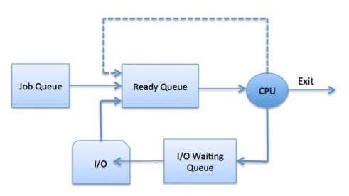
1. System processes
2. Interactive processes
3. Background processes
4. Batch process
5. CPU scheduling
6. Synchronize data transfer
7. Print spooler
8. First-come-first-serve (servers for example)

Ring buffer

Ring buffers are queues where the new data can overwrite the old data when needed. It’s like a queue implemented with an array, providing limited space. Problem that can occur if the pointer for adding new data reaches the pointer for fetching data, in other words the front pointer and the back pointer must never overlap.

Application of ring buffers

1. Chats
2. Real-time processing

Okasaki Queue

A queue implemented with 2 linked lists.

https://ucsd-progsys.github.io/liquidhaskell-tutorial/09-case-study-lazy-queues.html

Other interesting topic to research https://en.wikipedia.org/wiki/Persistent_data_structure

Trees

A tree is a hierarchical data structure. A tree has one root node (one starting element) and all other elements are children/grandchildren/etc. of this root element.

The root in the picture above is 2. Its children are 7 and 5. 5 is a child of the root 2 and also the parent of 9.

How does the tree stay connected

There are 2 ways to keep the Nodes in the tree connected.

1. Each parent has pointers to its children. (The classic widely used approach)
2. Each node has a pointer to its parent. (Not widely used in most algorithms, but still very useful in some particular problems)
3. 1 and 2 combined - Each node has pointers to its children and a pointer to its parent. This makes the traversal of the tree very easy in each direction, but also takes more memory.

Node of a binary tree

struct Node {
    int data;
    Node* left = nullptr;
    Node* right = nullptr;
};

Node of a tree with variable number of children

struct Node {
    int data;
    vector<Node*> children;
};

Traversals

Preorder (DFS)

Preorder traversal is also known as DFS (Depth First Search).

Time complexity , where n is the number of nodes in the tree.

The order in which we visit nodes is

1. Current node
2. Children of the node in order from left to right

void DFS(Node* current) {
    if (current == nullptr) {
        return;
    }
    
    cout << current->data; // do something with the node
    
    DFS(current->left);
    DFS(current->right);
}

Postorder

Time complexity , where n is the number of nodes in the tree.

The order in which we visit nodes is

1. Children of the node in order from left to right
2. Current node

void Postorder(Node* current) {
    if (current == nullptr) {
        return;
    }

    Postorder(current->left);
    Postorder(current->right);
    
    cout << current->data; // do something with the node
}

Inorder traversal

Time complexity , where n is the number of nodes in the tree.

The order in which we visit nodes is

1. Left child
2. Current node
3. Right child

void Postorder(Node* current) {
    if (current == nullptr) {
        return;
    }

    Postorder(current->left);
    cout << current->data; // do something with the node
    Postorder(current->right);
}

Level order

Level order is also known as WFS (Width First Search) or BFS (Breadth First Search).

Time complexity , where n is the number of nodes in the tree.

The order in which we visit nodes is

1. All the nodes of level 1 (the root)
2. All the nodes of level 2 from left to right (the children of the root)
3. All the nodes of level 3 from left to right
4. etc.

Morris order

Morris order is an inorder traversal algorithm which does not use extra space for recursion or a stack. However it changes the tree during traversal and then reverts it to its original state.

https://en.wikipedia.org/wiki/Tree_traversal#Morris_in-order_traversal_using_threading

Tree variations

Generalized tree

A tree where each node stores whatever data we need and has an arbitrary number of children.

struct Node {
	int data;
    std::vector<Node*> children;
}

Trie

Segment Tree

Merge Tree

K-D Tree

BSP Tree

Merkle Tree

Treap

Threaded Binary Tree

Strict Binary Tree

Full Binary Tree

Complete Binary Tree

Binary Search Trees

BST

A binary search tree is a tree with the following properties

1. Each node has at most 2 children (left and right)
2. The value of the left child of a node is smaller than the value of the parent
3. The value of the right child of a node is bigger than the value of the parent

struct BST {
    int data;
    BST* left;
    BST* right;
}

BST operation	Average case	Worst case
insert(key)
remove(key)
find(key)
findMin()
findMax()

The order in which we receive the data is important! If we receive ordered array [1, 2, 3, 4, ...] we will constantly add in the right subtree. Therefore we will hit the worst case per operation.

AVL Tree

AVL Tree is a BST tree which also has information on each node what is the height of the node. This allows it to balance itself and always keep the height as small as possible.

struct BST {
    int data;
    int height;
    BST* left;
    BST* right;
}

Complexity

BST operation	Average case	Worst case
insert(key)
remove(key)
find(key)
findMin()
findMax()

The order in which we receive the data doesn’t matter because the tree balances itself to always have the smallest possible height.

Balancing

Balancing is done using the height kept in the nodes. To use the height a Balance Factor (BF) is calculated on each node. . Depending on the value of the balance factor there are the following 2 situations:

1. - If the balance factor is between -1 and 1 then the node is balanced.
2. - if the balance factor less than -1 or more than 1 (e.g -2 or 2), the node is not balanced and we must balance it.

If a node is unbalanced we can have 4 rotations that we can do:

1. RR (Right Right) - For the current node the right subtree is heavier. For the right child of the current node the right subtree is heavier.
2. RL (Right Left) - For the current node the right subtree is heavier. For the right child of the current node the left subtree is heavier.
3. LL (Left Left) - For the current node the left subtree is heavier. For the left child of the current node the left subtree is heavier.
4. LR (Left Right) - For the current node the left subtree is heavier. For the left child of the current node the right subtree is heavier.

Code

Height and balance calculation

void calculateHeight() {
    height = 0;
    if (left) {
        height = max(height, left->height + 1);
    }
    if (right) {
        height = max(height, right->height + 1);
    }
}

int leftHeight() const {
    if (left) {
        return left->height + 1;
    }
    return 0;
}

int rightHeight() const {
    if (right) {
        return right->height + 1;
    }
    return 0;
}

void recalculateHeights() {
    if (left) {
        left->calculateHeight();
    }
    if (right) {
        right->calculateHeight();
    }
    this->calculateHeight();
}

int balance() const {
    return leftHeight() - rightHeight();
}

Rotations

void rotateRight() {
    if (!left) {
        return;
    }

    Node* leftRight = this->left->right;
    Node* oldRight = this->right;

    swap(this->data, this->left->data);
    this->right = this->left;
    this->left = this->left->left;
    this->right->left = leftRight;
    this->right->right = oldRight;
}

void rotateLeft() {
    if (!right) {
        return;
    }

    Node* rightLeft = this->right->left;
    Node* oldLeft = this->left;

    swap(this->data, this->right->data);
    this->left = this->right;
    this->right = this->right->right;
    this->left->left = oldLeft;
    this->left->right = rightLeft;
}

Check at each node when going up/down the recursion when inserting/deleting/etc.

void fixTree() {
    if (balance() < -1) { // Right is heavier
        if (right->balance() <= -1) { // RR
            this->rotateLeft();
            recalculateHeights();
        }
        else if (right->balance() >= 1) { // RL
            right->rotateRight();
            this->rotateLeft();
            recalculateHeights();
        }
    }
    else if (balance() > 1) { // Left is heavier
        if (left->balance() >= 1) { // LL
            this->rotateRight();
            recalculateHeights();
        }
        else if (left->balance() <= -1) { // LR
            left->rotateLeft();
            this->rotateRight();
            recalculateHeights();
        }
    }
}}

Modify insert

Node* _insert(int value, Node* current) {
	// insert from BST
    current->calculateHeight();
    current->fixTree();
    return current;
}

Modify remove

Node* _remove(int value, Node* current) {
	// remove from BST
    current->calculateHeight();
    current->fixTree();
    return current;
}

Splay Tree

Scape Goat Tree

Red-black Tree

2-3 Tree

Heap

Heap sort

Disjoint Set

Hashes

Rolling hash

Bloom Filter

Graphs

Graph variations

Undirected Graph

Directed Graph

Weighted Graph

Connected Graph

Disconnected Graph

Trees

Complete Graph

Tournament Graph

Bipartite Graph

Representing Graphs

Edge List

Adjacency Matrix

Adjacency List

Exploring Graphs

Depth First Search

Breadth First Search

Topological Sorting

Minimum Spanning Tree

Prim

Kruskal

Shortest Path

Dijkstra

Bellman-Ford

A*

NP-problems