Election
Having seen this page at Indiemapper, I was interesting in seeing if a similar map could be produced in R using ggplot2. I’ve detailed what I did, with the code inline. The full code listing is available here. (Though not the data, links are available below for that.)
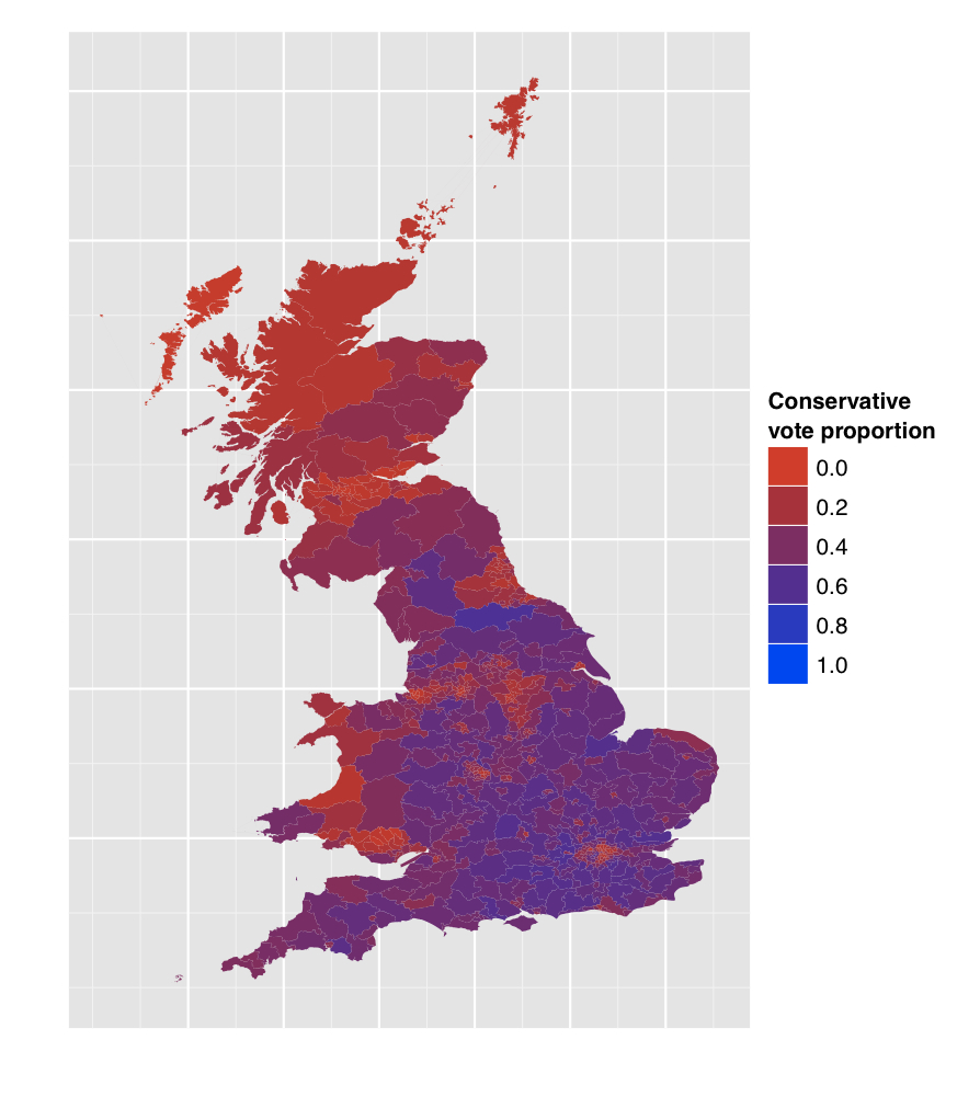
The map looks like this:
How did I make it?
Unfortunately the data is not open licensed, so I’m afraid you’ll have to get that yourselves. First, the Ordinance Survey data. Having downloaded and unzipped this, there should be a folder called “Boundary-Line Oct 2010 data”, in that you want the files:
Boundary-Line\ October\ 2010/Boundary-Line\ Oct\ 2010/data/westminster_const_region.*
These are the shape files that define the boundaries of the UK constituencies. You’ll note at this point that they are quite large (about 65MB), trimming them down to size is going to be a major part of the work.
The data can be loaded with the shapefiles library:
library(shapefiles)
# load the Westminster constituency shapefiles...
# this takes a LONG TIME
shapefile<-read.shapefile("westminster_const_region")
# the constituency shapes are in shapefile[[1]][[1]][[1:632]]$points
# list of constituencies
constituencies<-shapefile[[1]][[1]]
# and their names
os.names<-shapefile$dbf$dbf$NAME
Now we have the geographic data, the need the polling data. This is available from the Guardian Data Blog as a Google spreadsheet here, you can export this from Google Docs as a CSV file that R can read.
votes<-read.csv("uk_election.csv",header=TRUE)
con.voteshare<-votes$CON_PER/100 # Tory vote share in (0,1)Unfortunately the Guardian and the OS have a different idea of what constituencies should be called (this is mainly because the Guardian’s list is designed so it’s easy to find your constituency). This leads to a rather extensive set of regular expressions to rename the constituencies (or, rather to create a lookup table between the two sets).
##############################
# map between the two sets of names for constituencies!

# there was no election in Thirsk and Malton because John Boakes died
# so it does not appear in the Guardian figures

guardian.names<-as.vector(votes$CONSTITUENCY)
guardian.names<-c(guardian.names,"Thirsk and Malton")

# first get rid of "Co Const" from the end of all of the
# OS names
os.names<-gsub(" Co Const","",os.names)
os.names<-gsub(" Boro Const","",os.names)
os.names<-gsub(" Burgh Const","",os.names)


# do "x, city of"
guardian.names<-gsub("(\\w+), City of$","City of \\1",guardian.names,perl=TRUE)
# do "x, The"
guardian.names<-gsub("(\\w+), The$","The \\1",guardian.names,perl=TRUE)
guardian.names<-gsub("St (\\w*)","St. \\1",guardian.names,perl=TRUE)
guardian.names<-gsub("(\\w+) Under (\\w+)$","\\1-under-\\2",guardian.names,perl=TRUE)
guardian.names<-gsub("Hull (\\w*)","Kingston upon Hull \\1",guardian.names,perl=TRUE)

# match up the easy names
mapper<-match(guardian.names,os.names)

# geography - switch NSEW etc
guardian.names[which(is.na(mapper))]<-gsub("(\\w+) North East$","North East \\1",guardian.names[which(is.na(mapper))],perl=TRUE)
guardian.names[which(is.na(mapper))]<-gsub("(\\w+) South East$","South East \\1",guardian.names[which(is.na(mapper))],perl=TRUE)
guardian.names[which(is.na(mapper))]<-gsub("(\\w+) North West$","North West \\1",guardian.names[which(is.na(mapper))],perl=TRUE)
guardian.names[which(is.na(mapper))]<-gsub("(\\w+) South West$","South West \\1",guardian.names[which(is.na(mapper))],perl=TRUE)
mapper<-match(guardian.names,os.names)
guardian.names[which(is.na(mapper))]<-gsub("(\\w+) East$","East \\1",guardian.names[which(is.na(mapper))],perl=TRUE)
guardian.names[which(is.na(mapper))]<-gsub("(\\w+) West$","West \\1",guardian.names[which(is.na(mapper))],perl=TRUE)
mapper<-match(guardian.names,os.names)
guardian.names[which(is.na(mapper))]<-gsub("(\\w+) North$","North \\1",guardian.names[which(is.na(mapper))],perl=TRUE)
guardian.names[which(is.na(mapper))]<-gsub("(\\w+) South$","South \\1",guardian.names[which(is.na(mapper))],perl=TRUE)
guardian.names[which(is.na(mapper))]<-gsub("(\\w+) Mid$","Mid \\1",guardian.names[which(is.na(mapper))],perl=TRUE)
guardian.names[which(is.na(mapper))]<-gsub("(\\w+) Central$","Central \\1",guardian.names[which(is.na(mapper))],perl=TRUE)
mapper<-match(guardian.names,os.names)

# commas
guardian.names[which(is.na(mapper))]<-gsub("(Liverpool|Birmingham|Brighton|Sheffield|Manchester|Plymouth|Southampton|Enfield|Ealing|Lewisham) (\\w*)","\\1, \\2",guardian.names[which(is.na(mapper))],perl=TRUE)

# Devon
guardian.names<-gsub("Devon West and Torridge","Torridge and West Devon",guardian.names)
mapper<-match(guardian.names,os.names)

# awkward
awkward<-guardian.names[which(is.na(mapper))]
awkward<-gsub("(\\w+) (West|South|Central|North|East|Mid) and (\\w+)","\\2 \\1 and \\3",awkward)
guardian.names[which(is.na(mapper))]<-awkward

# DONE!
mapper<-match(guardian.names,os.names)

# now have the vector mapper which goes FROM guardian names TO OS names
# guardian.names[20] == os.names[629] => mapper[20]==629

# for fun let's also go the other way
bmapper<-match(1:632,mapper)The second issue is that the OS map is incredibly high resolution. Each of the constituencies is made up of one (or more) polygons. The smallest (terms of the number of points that define it) constituency is Islington South and Finsbury with 339 points, the largest with 362,590 points is Orkney and Shetland. As you might imagine, plotting a polygon defined by over 360,000 points takes a long time, so it’s important to simplify the polygons.
There are some smart ways of reducing the complexity of regions in maps, however (as far as I can see) they do not have implementations in R. So I just reduced the number of points to a quarter of the original number, per constituency using a seq() statement to drop the points systematically.
list_to_coords<-function(these.coords,i,codei){
   # do something here to cut down on number of points
   fact<-0.25 # fraction of the points to keep
   n.coords<-length(these.coords$X)
   this.seq<-c(1,seq(2,n.coords-1,length=floor(n.coords*fact)),n.coords)
   these.coords<-these.coords[this.seq,]

   nreps<-length(these.coords$X)
   this.row<-data.frame(x=these.coords$X,
                        y=these.coords$Y,
                        name=rep(os.names[i],nreps),
                        code=rep(i,nreps),
                        group=rep(codei,nreps),
                        votes=rep(con.voteshare[bmapper[i]],nreps))
   return(this.row)
}
Some of the constituencies are very (very) big! So let’s pre-chop them by getting rid of some of their islands. The 7 biggest are:
- Banff and Buchan
- St. Ives
- Ross, Skye and Lochaber
- Caithness, Sutherland and Easter Ross
- Argyll and Bute
- Orkney and Shetland
- Na h-Eileanan an Iar (formerly the Western Isles)
So let’s chop them down:
too.big<-c(619, 610, 613, 612, 617, 615, 616)
for(i in too.big){
   constituencies[[i]]$num.parts<-25
   constituencies[[i]]$parts<-constituencies[[i]]$parts[1:26]
   X<-constituencies[[i]]$points$X[1:constituencies[[i]]$parts[26]]
   Y<-constituencies[[i]]$points$Y[1:constituencies[[i]]$parts[26]]
   constituencies[[i]]$points<-NULL
   constituencies[[i]]$points<-data.frame(X=X,Y=Y)
}I used ggplot2 to create the map, first putting all this data into a data.frame with the structure:
bigframe<-data.frame(x=NA,y=NA,name=NA,code=NA,group=NA,votes=NA)which correspond to one line per point in each polygon. Along with each \(x\) and \(y\) coordinate, also recorded are: the name of the constituency, the number of that constituency, a group code (which is different for each polygon in the full map, so that islands are separate) and finally the proportion of votes for the Conservative party.
So, filling up that data.frame, we have the following (rather inefficient) piece of code:
for(i in 1:length(constituencies)){

   parts<-c(constituencies[[i]]$parts,length(constituencies[[i]]$points$X))

   # do something nice with multiple parts
   if(constituencies[[i]]$num.parts>1){

      parts<-c(constituencies[[i]]$parts,length(constituencies[[i]]$points$X))

      for(p.ind in 1:constituencies[[i]]$num.parts){
         these.coords<-constituencies[[i]]$points[parts[p.ind]:(parts[(p.ind+1)]-1),]

         bigframe<-rbind(bigframe,list_to_coords(these.coords,i,codei))
         codei<-codei+1
      }
   }else{
      p.ind<-length(constituencies[[i]]$points$X)
      these.coords<-constituencies[[i]]$points[1:p.ind,]

      bigframe<-rbind(bigframe,list_to_coords(these.coords,i,codei))
      codei<-codei+1
   }
}
bigframe<-bigframe[-1,]
(If you have a suggestion of how to make this quicker, I’d be really interested!)
As noted above, John Boakes (UKIP candidate) died shortly before polling day , so the election for Thirsk and Malton was posponed until 27 May 2010. Also, the speaker is not included in the data above; strictly speaking, the speaker renounces his party but he ran for election has a Conservative, so we include him here. So filling those two gaps:
bigframe$votes[bigframe$code==89]<-47.3/100
bigframe$votes[bigframe$code==523]<-52.9/100
With that done we can create the map!
# constituency polygons
con.geom<-geom_polygon(aes(x=x, y=y, fill=votes, group=group), data=bigframe)

# do the plotting
p<-ggplot()
p<-p+con.geom
p<-p+scale_fill_continuous(low="red",high="blue",limits=c(0,1))
print(p)