Profiling and metrics
#GPU Kernels Here I will detail the profiling results of EPIC's first Bifrost-based iteration. Briefly, the EPIC code creates a pipeline where the data streams move through multiple processing (or Operating) blocks (e.g., `DecimationOp) via ring buffers. Based on the user-specified settings, the EPIC program may produce images up to a bandwidth of 3.3 MHz at all four (XX, YY, XY, YX) polarizations. Each Op-block is run on a separate thread, bound to its own CPU, while the entire process currently utilizes only one of the two available GPUs on the EPIC node at SV. Below I will only describe results pertaining to the GPU and I will post CPU profiling on a separate thread.
Before I show the results, I will describe the tools used. I used NVIDIA Nsight Systems to measure the overall performance (or system-level profiling for the GPU-peeps), and NVIDIA Nsight Compute to measure the kernel metrics. See Pearson (2020) for a nice overview of these tools. For both tools, I ran EPIC with the following options to profile the code with a total runtime of 50 s:
- Gulp size 40 ms (or
--nts 1000) - Single polarization
- Image size 64x64
- Image resolution 1.8 deg
- Accumulation time (80 ms)
- Channels 90
Run command:
LD_PRELOAD="libvma.so" VMA_RX_POLL=1000 VMA_INTERNAL_THREAD_AFFINITY=0 VMA_RX_PREFETCH_BYTES=128\
 VMA_THREAD_MODE=0 VMA_MTU=9000 VMA_TRACELEVEL=0 numactl --cpubind=1 --membind=1\
 ./LWA_bifrost.py  --addr 239.168.40.16 --port 4015 --channels 90\
--imagesize 64 --imageres 1.8 --accumulate 80 --nts 1000 --singlepol --duration 50The imaging takes place in the MOFFCorrelatorOp block, which mostly operates on the GPU. For completeness, I list the other main blocks in the imager in the actual sequence.
- FEngineOp (CPU): This block captures packets from the F-Engines and orders them accordingly.
- DecimationOp (CPU or GPU): The channels may be averaged (GPU) or filtered (CPU) for further processing.
- MoFFCorrelatorOp
- SaveOp (CPU): Formats and saves the images to disk or PostgresDB
Following is a brief outline of the sequence of operations that are carried out in this block. The typical processing times for a 40 ms gulp are provided in square brackets. I will introduce autocorrelation removal in a different profiling run.
- Memset the cross-multiplied data to 0 (once per image)   [5.0  ms]
Loop until accumulation>=80 ms
 - Load antenna (or un-gridded) data                       [1.9  ms]
 - Memset the gridded data to 0                            [5.0  ms]
 - Grid the data (VGrid kernel)                            [2.7  ms]
 - Inverse FFT the gridded data (vec_2d_fft kernel)        [11.0 ms]
 - Cross multiply (XGrid kernel)                           [16.6 ms]
- Combine all images in the gulp (reduce kernel)           [5.0  ms]
-                                              Total time: [42.2 ms]
The total time to image two 40 ms gulps is therefore 42.2 * 2 + 5 = 89.4 ms. The final image has dimensions of [2 (real, complex), npol, nchan, grid_size, grid_size].
Below is a screenshot from the Nsight systems UI. The data is available in the profiling/systems folder of the repo. See the user guide for information on how to interpret the data.
Notice the ~4 ms gap between reduce kernel and
D2Hcopy of the reduced image. I'm unsure what is causing this, but I presume it is the time required to acquire a lock on the output ring buffer, which is an input to theSaveOpblock. Although it could be a gap introduced by the profiler, it is unlikely for the gap to consistently exist only between the reduce and the copy steps.
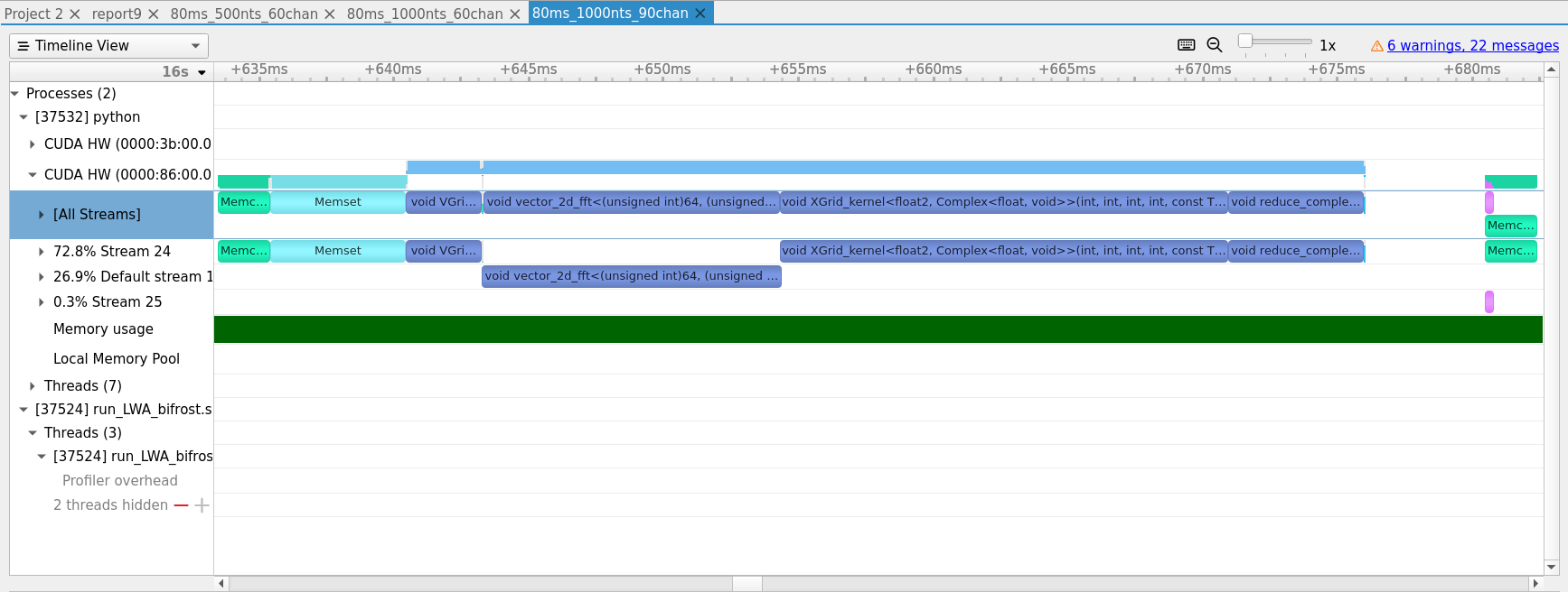
Although the FFT kernel runs in a different stream than VGrid and XGrid, they do not overlap. Furthermore, the FFT and the XGrid kernels appear to be the hotspots in imaging. To see if there is room for any improvement, let's take a look at the profiling results from Nsight Compute. I used the same options provided above to run the EPIC imager. See Subrahmaniam (2021) for a nice lecture on how to use Nsight Systems and Compute to optimize kernels. Below I will describe the main takeaways for each kernel except for the reduce kernel, which, for unknown reasons, does not show up in Compute's profiling.
The below figure shows that the kernel is bandwidth-bound and that memory is more heavily utilized than compute SMs. That means, for a given unit of memory bandwidth utilization, non-optimal work is being done. This can be seen in the figure below.
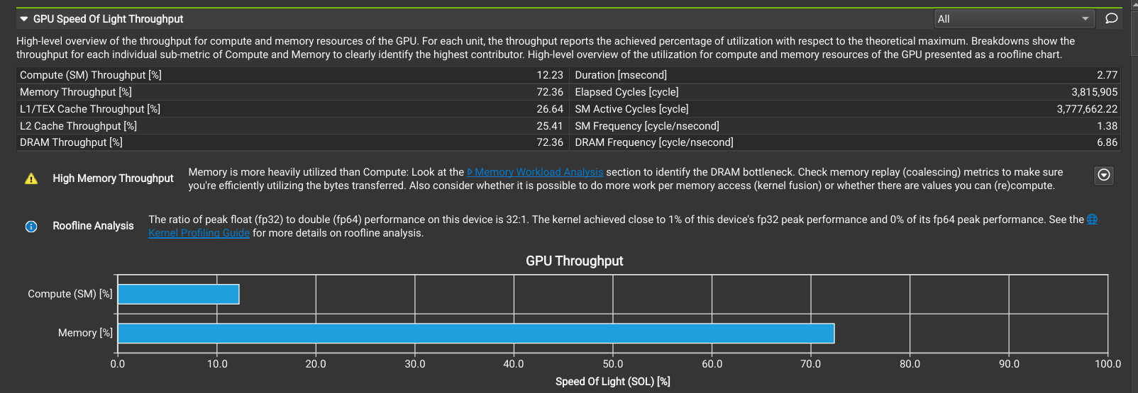
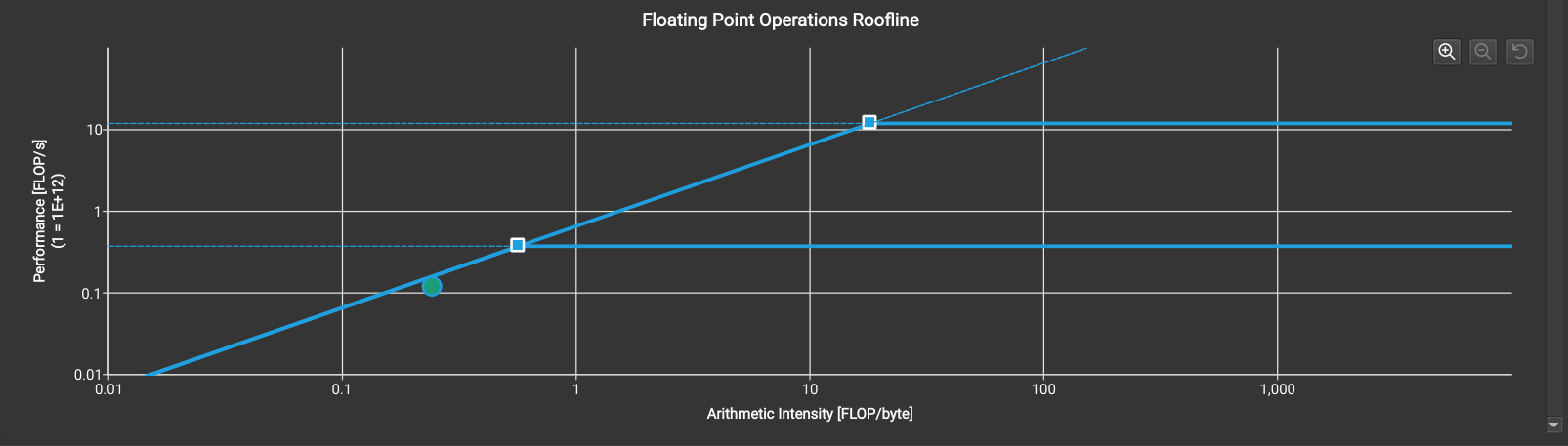
The first roofline in the above figure indicates the peak double-precision performance, while the second one indicates the peak single-precision performance. The achieved performance is shown as a filled-green circle that is about half of the peak double-precision performance. Note that the kernel achieves nearly 100% warp occupancy (see figure below). Put another way, it keeps the GPU fully occupied during the computation, however, does not achieve a high FLOPS/byte. It is because the kernel spends most of the time accessing memory inefficiently resulting in uncoalesced global memory accesses.

TODO: Improve global memory accesses in VGrid. However, note that this step only takes about 7% of the total process time, and hence should be prioritized below the rest.
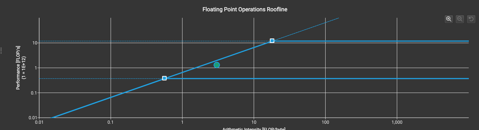
The FFT kernel is also bandwidth bound similar to the VGrid kernel. The FLOPS/bytes (3.06) is higher than the expected double-precision roofline (0.57) suggesting the amount of work done per byte is near the optimal value.
The theoretical warp occupancy (fraction of the total available active warps occupied) is, however, only 50%. It is because the shared memory required by all the active warps is greater than the available memory (see figure below) that is restricting the warp occupancy to 50%.


Furthermore, the above figure shows that the warp occupancy can be improved by increasing block size.
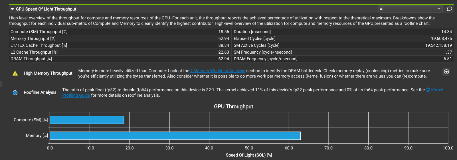
XGrid, although bandwidth bound similarly to XGrid and FFT, it has as >80% bandwidth usage (see figure below).
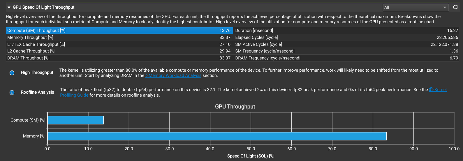
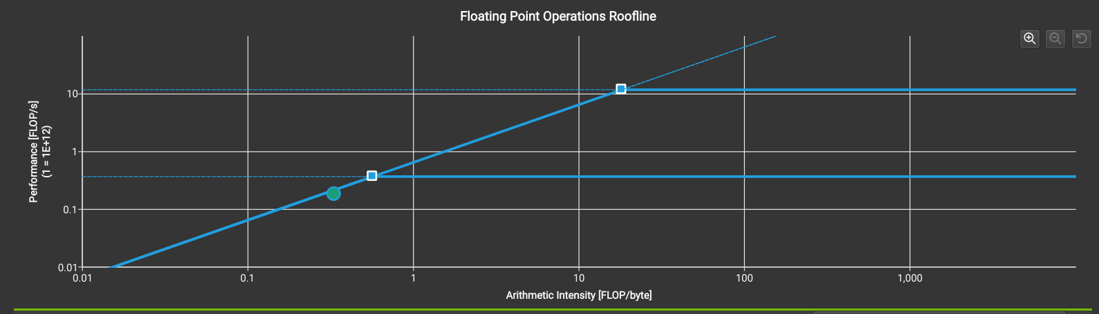
The peak performance is about half of the expected peak double-precision performance (fig above). Both these metrics suggest that we can improve the SM throughput by shifting the work from a different kernel into XGrid.
The main intent of these profiling runs is to understand the hotspots in the EPIC imager and multiple ways where we may be able to optimize the imager have been identified. While FFT and XGrid appear to be the main hotspots, the high memory throughput compared to lower SM throughput in all the kernels suggests that the total runtime can be reduced by coalescing these kernels. This will be different from launching these kernels in sequence using streams that operate on chunks of the data simultaneously. Both methods must be compared to determine the best possible approach.
While the current profiling is exclusive to the GPU, CPU profiling is necessary to understand the impact of ring buffers and whether we need to switch to lock-free ring buffers.
TODO: expand this section