omicsplot

Publication-quality matplotlib figures for omics data, with two focuses:

• omicsplot.heatmap — ComplexHeatmap-style heatmaps where the body is specified in absolute physical units (mm, cm, inch, pt). Surrounding panels (dendrograms, annotations, labels, colorbar, legend) grow outward without shrinking the body. Multi-panel composition with | (side-by-side) and / (stacked) keeps body positions exactly aligned across panels. Includes a chromosome-aware genomic_heatmap for binned signals (methylation, expression, copy number, accessibility).

• omicsplot.tracks — genome-wide track plots stacked vertically across per-chromosome subplot axes sized proportionally to chromosome lengths. Built-in track types: scatter, line segments, bar, step coverage, SV triangles. Trivially extensible by subclassing _BaseTrack.

Both submodules share a unit system inspired by R's grid::unit(): absolute (mm, cm, inch, pt), relative (npc), and flexible (null).

Install

pip install omicsplot

Requires Python ≥ 3.10. Depends on numpy, pandas, matplotlib, scipy, seaborn.

Quick start

The snippets below show the API for each value proposition. Complete runnable examples — including synthetic data generation — are in docs/scripts/render_readme.py, which produces the figures shown here.

Heatmap with absolute physical sizing

from omicsplot import unit
from omicsplot.heatmap import Heatmap, HeatmapAnnotation

hm = Heatmap(
    df,
    width=unit(120, 'mm'),
    height=unit(50, 'mm'),
    row_dendrogram_size=unit(12, 'mm'),
    col_dendrogram_size=unit(10, 'mm'),
    z_score=0,                 # row-wise normalization
    cmap='RdBu_r',
    center=0,
)
hm.add_top_annotation(HeatmapAnnotation(
    group=sample_groups,
    batch=sample_batch,
    height=unit(3, 'mm'),
))
hm.draw()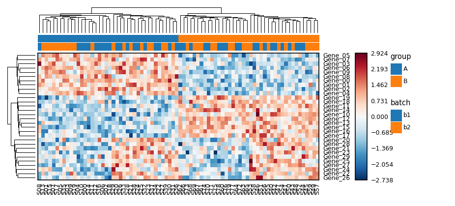

Multi-panel composition

Use | for side-by-side and / for stacked. With share_row_order=True (side-by-side) or share_col_order=True (stacked), bodies stay aligned across panels.

hm_a = Heatmap(mat_a, width=unit(40, 'mm'), height=unit(45, 'mm'),
               cmap='RdBu_r', center=0, name='Expression',
               show_row_names=False)
hm_a.add_left_annotation(HeatmapAnnotation(
    Group=groups, colors=group_colors, width=unit(4, 'mm'),
))

hm_b = Heatmap(mat_b, width=unit(25, 'mm'), height=unit(45, 'mm'),
               cmap='YlOrRd', col_cluster=False, name='Copy number',
               show_row_names=False)

(hm_a | hm_b).draw(share_row_order=True)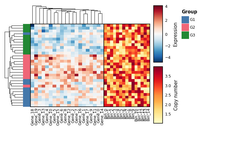

Compound layouts also work: (A | B) / C, A | B | C, etc.

Chromosome-aware genomic heatmap

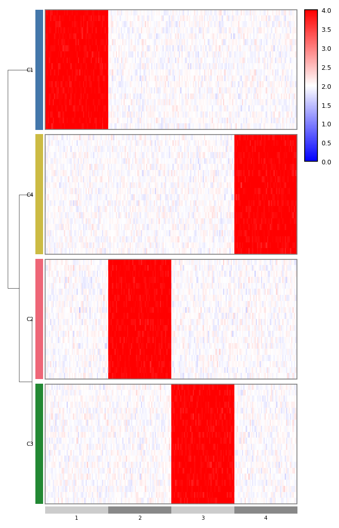
genomic_heatmap takes a long-form matrix with chrom/start/end columns and arranges the columns into chromosome-proportional segments. The optional cluster-of-clusters dendrogram (row_cluster_dendrogram) shows relationships between groups, not individual rows.

from omicsplot.heatmap import genomic_heatmap

genomic_heatmap(
    matrix,                    # columns: chrom, start, end, then per-cell
    chrom_col='chrom',
    cmap='bwr', vmin=0, vmax=4, center=2,
    row_cluster=False,
    show_row_names=False,
    row_annotation={'Cluster': cluster_labels},
    row_annotation_colors={'Cluster': palette},
    row_gap=unit(2, 'mm'),
    row_cluster_dendrogram=cluster_link,             # leaves are groups
    row_cluster_dendrogram_size=unit(10, 'mm'),
)

Genome-wide tracks

Each chromosome gets its own subplot axis sized proportionally to its length. genome_range returns chromosome lengths for common builds.

from omicsplot import genome_range
from omicsplot.tracks import ScatterTrack, plot_tracks

gs = genome_range(genome='hg38')

scatter = ScatterTrack(
    points, x_column='start', y_column='value',
    ylabel='logR', ylim=(-1.5, 1.5),
    s=1, alpha=0.4,
)
plot_tracks(scatter, gs, figsize=(10, 0.8))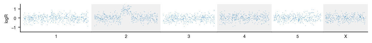

Status

Alpha. API may change before 1.0.

License

MIT.