Data-Science---Module-9-Assignment

Module 9: Intro to Logistic Regression

Install packages if you have not previously used them.

install.packages("titanic") install.packages("caTools") install.packages("caret") install.packages("e1071") ## dependency for confusion matrix. install.packages("dplyr")

Load packages

library(titanic) # contains the data set library(caTools) # contains function for splitting the data library(caret) # contains function for creating a confusion matrix library(dplyr) # data manipulation library(e1071)

Access titanic_train data set from the {titanic} package and call it titanic_data

titanic_data <- titanic::titanic_train

Rename the columns to only use lower case letters

names(titanic_data) <- tolower(names(titanic_data))

Explore the data frame object

glimpse(titanic_data)

glimpse(titanic_data) Observations: 891 Variables: 12 $ passengerid 1, 2, 3, 4, 5, 6, 7, 8, 9, 10, 11, 12, 13, 14, 1… $ survived 0, 1, 1, 1, 0, 0, 0, 0, 1, 1, 1, 1, 0, 0, 0, 1, … $ pclass 3, 1, 3, 1, 3, 3, 1, 3, 3, 2, 3, 1, 3, 3, 3, 2, … $ name "Braund, Mr. Owen Harris", "Cumings, Mrs. John B… $ sex "male", "female", "female", "female", "male", "m… $ age 22, 38, 26, 35, 35, NA, 54, 2, 27, 14, 4, 58, 20… $ sibsp 1, 1, 0, 1, 0, 0, 0, 3, 0, 1, 1, 0, 0, 1, 0, 0, … $ parch 0, 0, 0, 0, 0, 0, 0, 1, 2, 0, 1, 0, 0, 5, 0, 0, … $ ticket "A/5 21171", "PC 17599", "STON/O2. 3101282", "11… $ fare 7.2500, 71.2833, 7.9250, 53.1000, 8.0500, 8.4583… $ cabin "", "C85", "", "C123", "", "", "E46", "", "", ""… $ embarked "S", "C", "S", "S", "S", "Q", "S", "S", "S", "C"…

Note: In the survived column, 0 indicates death, 1 indicates survival

Change pclass and sex columns to factors

titanic_data <- titanic_data %>% mutate(pclass = as.factor(pclass), sex = as.factor(sex))

glimpse(titanic_data) Observations: 891 Variables: 12 $ passengerid 1, 2, 3, 4, 5, 6, 7, 8, 9, 10, 11, 12, 13, 14, 1… $ survived 0, 1, 1, 1, 0, 0, 0, 0, 1, 1, 1, 1, 0, 0, 0, 1, … $ pclass 3, 1, 3, 1, 3, 3, 1, 3, 3, 2, 3, 1, 3, 3, 3, 2, … $ name "Braund, Mr. Owen Harris", "Cumings, Mrs. John B… $ sex male, female, female, female, male, male, male, … $ age 22, 38, 26, 35, 35, NA, 54, 2, 27, 14, 4, 58, 20… $ sibsp 1, 1, 0, 1, 0, 0, 0, 3, 0, 1, 1, 0, 0, 1, 0, 0, … $ parch 0, 0, 0, 0, 0, 0, 0, 1, 2, 0, 1, 0, 0, 5, 0, 0, … $ ticket "A/5 21171", "PC 17599", "STON/O2. 3101282", "11… $ fare 7.2500, 71.2833, 7.9250, 53.1000, 8.0500, 8.4583… $ cabin "", "C85", "", "C123", "", "", "E46", "", "", ""… $ embarked "S", "C", "S", "S", "S", "Q", "S", "S", "S", "C"…

Split the data into training set (80%) and testing set (20%)

set.seed(123) # ensure reproducibility sample <- sample.split(titanic_data$passengerid, SplitRatio = .80) train <- titanic_data[sample == TRUE,] test <- titanic_data[sample == FALSE,]

Apply a logistic model using sex and pclass to predict survived using the train set

logreg <- glm(formula = survived ~ pclass + sex, family = binomial(link = "logit"), data = train)

Generate predictions applying the test set data to the logreg model and store in column called prediction

test <- test %>% mutate(prediction = predict(logreg, newdata = test, type = "response"))

Update the prediction column by applying a decision rule: if prediction > 0.5, change it to 1, else change it to 0

test <- test %>% mutate(prediction = ifelse(prediction > 0.5, 1, 0))

Change prediction and survived columns to factors

test <- test %>% mutate(prediction = as.factor(prediction), survived = as.factor(survived))

Create and print confusion matrix

confusion_matrix <- confusionMatrix(data = test$prediction, reference = test$survived) confusion_matrix

confusion_matrix Confusion Matrix and Statistics Reference Prediction 1 0 1 48 17 0 22 92
Accuracy : 0.7821
95% CI : (0.7144, 0.8402) No Information Rate : 0.6089
P-Value [Acc > NIR] : 6.083e-07
Kappa : 0.5366
Mcnemar's Test P-Value : 0.5218
Sensitivity : 0.8440
Specificity : 0.6857
Pos Pred Value : 0.8070
Neg Pred Value : 0.7385
Prevalence : 0.6089
Detection Rate : 0.5140
Detection Prevalence : 0.6369
Balanced Accuracy : 0.7649
'Positive' Class : 0

Summarize the model

summary(logreg)

summary(logreg) Call: glm(formula = survived ~ pclass + sex, family = binomial(link = "logit"), data = train) Deviance Residuals: Min 1Q Median 3Q Max
-2.1234 -0.7326 -0.4657 0.6483 2.1332
Coefficients: Estimate Std. Error z value Pr(>|z|)
(Intercept) 2.1435 0.2402 8.926 < 2e-16 *** pclass2 -0.6905 0.2710 -2.548 0.0108 *
pclass3 -1.6791 0.2358 -7.121 1.07e-12 *** sexmale -2.6313 0.2027 -12.979 < 2e-16 ***

---

Signif. codes: 0 ‘’ 0.001 ‘’ 0.01 ‘’ 0.05 ‘.’ 0.1 ‘ ’ 1 (Dispersion parameter for binomial family taken to be 1) Null deviance: 947.02 on 711 degrees of freedom Residual deviance: 673.57 on 708 degrees of freedom AIC: 681.57 Number of Fisher Scoring iterations: 4

1. A hypothesis test rejects the null hypothesis (H0) if the resulting p-value is less than a predefined value of alpha (typically 0.05). However, this may lead to Type 1 and Type 2 errors. The confusion matrix below demonstrates how the predicted values and the observed values are interpreted to identify Type 1 and Type 2 error. Observed True Observed False Predicted True True Positive False Positive (Type 2 Error) Predicted False False Negative (Type 1 Error) True Negative Confusion Matrix and Statistics Reference Prediction 1 0 1 48 17 0 22 92
   Accuracy : 0.7821
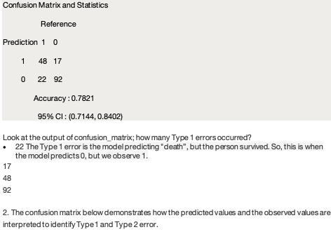
   95% CI : (0.7144, 0.8402) Look at the output of confusion_matrix; how many Type 1 errors occurred? • 22 The Type 1 error is the model predicting "death”, but the person survived. So, this is when the model predicts 0, but we observe 1. • 17 • 48 • 92

2. The confusion matrix below demonstrates how the predicted values and the observed values are interpreted to identify Type 1 and Type 2 error. Observed True Observed False Predicted True True Positive False Positive (Type 2 Error) Predicted False False Negative (Type 1 Error) True Negative Confusion Matrix and Statistics Reference Prediction 1 0 1 48 17 0 22 92
   Accuracy : 0.7821
   95% CI : (0.7144, 0.8402) Look at the output of confusion_matrix; how many Type 2 errors occurred? • 17 The model is predicting survival, but the passenger died; this occurs when the model prediction is 1, but the observation is 0 • 42 • 92 • 22

Question 3: What is the overall accuracy of the model when applied to the test data set? Confusion Matrix and Statistics Reference Prediction 1 0 1 48 17 0 22 92
Accuracy : 0.7821
95% CI : (0.7144, 0.8402) 0.7296 To calculate this value, subtract the proportion of incorrect predictions from 1: 1 - (17 + 22) / 179 Question 4: Look at the summary of the model. Which is the correct interpretation of the model coefficients?

summary(logreg) Call: glm(formula = survived ~ pclass + sex, family = binomial(link = "logit"), data = train) Deviance Residuals: Min 1Q Median 3Q Max
-2.1234 -0.7326 -0.4657 0.6483 2.1332
Coefficients: Estimate Std. Error z value Pr(>|z|)
(Intercept) 2.1435 0.2402 8.926 < 2e-16 *** pclass2 -0.6905 0.2710 -2.548 0.0108 *
pclass3 -1.6791 0.2358 -7.121 1.07e-12 *** sexmale -2.6313 0.2027 -12.979 < 2e-16 ***

---

Signif. codes: 0 ‘’ 0.001 ‘’ 0.01 ‘’ 0.05 ‘.’ 0.1 ‘ ’ 1 (Dispersion parameter for binomial family taken to be 1) Null deviance: 947.02 on 711 degrees of freedom Residual deviance: 673.57 on 708 degrees of freedom AIC: 681.57 Number of Fisher Scoring iterations: 4 • sexmale looks to be the strongest coefficient • With all other factors equal, class 3 passengers had a higher chance of death than class 2 or class 1 passengers • Women have a higher chance of survival than men.

Question 5: Look at the summary of the model, particularly the output associated with class 2 passengers (pclass2). Calculate the 95% confidence interval around the estimated coefficient (-0.6905). Use the function confint(logreg) to find the confidence intervals. Select all of the following statements that are true.

confint(logreg) 2.5 % 97.5 % (Intercept) 1.684838 2.6268713 pclass2 -1.226216 -0.1625688 pclass3 -2.148562 -1.2228936 sexmale -3.037857 -2.2420780 exp(confint(logreg)) 2.5 % 97.5 % (Intercept) 5.39157945 13.8304315 pclass2 0.29340072 0.8499576 pclass3 0.11665178 0.2943771 sexmale 0.04793751 0.1062375

Q: For the 5th question in the Assignment one of the option is "The confidence interval shows that the true effect of this coefficient may be zero." How do we determine this, if there is a true effect or not. I know that we could say if a predictor has any relation to output variable with either z-score or p-value. But I do not understand on how to say if a coefficient has any effect or not. A: Consider a scenario where we have an odds of 1.0; here, the probability that this individual belongs in group 1 (i.e. makes > 50K) is 0.5, or 50%. If the confidence interval around that odds value has a lower limit of 0.85 and an upper limit of 1.15, the lower limit would tell us that the person has a ~46% probability of making >50K; which would result in an overall negative classification (i.e. "this person is predicted to not make >50K") and the upper limit would tell us that the person has a ~53.5% probability of making >50K; which would result in an overall positive classification (i.e. "this person is predicted to make >50K). Since these are two opposite results, we can't be confident that this predictor is at all useful for our goal of classifying income, and we would likely want to remove it as a predictor from our model.

Q: Why do we need to use exp, despite we can compare the coefficients without any conversion?

A: While you absolutely may compare the non-transformed predictions, these value represent the log odds, which is (generally speaking) not particularly meaningful to the average person. Instead, we typically talk about these results in either the context of "odds" (which is found as odds = exp(log odds)) or as "probability" (which is found as probability = odds / (1 + odds)). Which of these is communicated varies by field of study; in science, we typically report values in the context of probability, but in business it may be more common to report the values in the context of odds. As a quick example of how to convert these values: if the reported log odds is 0.974, then the odds are (approx) exp(0.974) = 2.65 and the probability is (approx) 2.65/(1+2.65) = 0.73

6. Which of the following statements is true about AIC? A lower value of AIC implies that the quality of the model is better. This estimator accounts for the number of parameters in the model. That's correct! A lower value of AIC implies that the quality of the model is better. This estimator accounts for the number of parameters in the model.

7. There are a number of regression methods in the generalized linear model family (GLM), what family do we use in the R code when creating a logistic regression model? glm(formula, family = “binomial”, data) That's correct! The correct family for a logistic regression model is the binomial.

8. Which below is used to help you decide which subset of inputs might be possible predictors for your model? That is particularly useful when you have LOTS of variables to choose from. Stepwise Regression That's correct! Stepwise regression is a great starting point for determining a subset of variables from a larger population of potential variables.

9. Below is the exponentiated coefficients from the reg2 model in lecture. We were looking at predictors of income. Which of the following statements is true about this output?

If you didn’t finish high school, your odds of making a higher salary are much lower. That's correct! When someone doesn’t finish high school, their odds of being in the higher income bracket are .1299 to 1 compared to those with more education.

10. What probability distribution is used to determine the p-value for independent variables in logistic regression? No, not quite! Z-scores are used to calculate the p-values, and these come from the Normal Distribution. Not Chi-Square nor Binomial for the independent variables