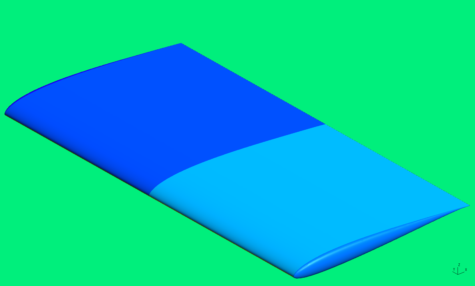
Wing
In this tutorial, we will cover generating a high order mesh for a wing with aspect ratio = 2 and a SD7003 airfoil section. While MeshOpt can generate the boundary layer for this case, it is better to use GMSH's boundary layer since MeshOpt is inefficient in creating 3D boundary layers. In this example, we will tell GMSH to generate a boundary layer containing only one layer of prismatic elements. This is not always guaranteed to work, but is a good workaround for some cases.
The geometry definition for this case is contained in the file SD7003Rectangular.stp in the Demo/Wing directory. The contents of the GMSH configuration file are copied below.
fflc = 10.0;
surf_len = 0.03;
lete_factor = 0.25;

Mesh.CharacteristicLengthMax = fflc;
Mesh.CharacteristicLengthExtendFromBoundary = 0;
Mesh.SaveParametric = 1;
Merge "SD7003Rectangular.stp";

Mesh.Algorithm = 7;


Physical Line(0) = {1:29};

Physical Surface(6) = {1:6};
Physical Surface(7) = {7:14};

Delete{ Volume{1:2}; }

Reverse Surface{7:14};

Surface Loop(100) = {1:6};
Surface Loop(101) = {7:14};

Volume(1) = {100,-101};
Physical Volume(0) = {1};

Field[2] = Box;
Field[2].VOut = fflc;
Field[2].VIn = 0.5*surf_len;
Field[2].XMax = 1.02;
Field[2].XMin = 0.98;
Field[2].YMax = 2.02;
Field[2].YMin = 1.6;
Field[2].ZMax = 0.35;
Field[2].ZMin = -0.01;

Field[5] = Box;
Field[5].VOut = fflc;
Field[5].VIn = surf_len;
Field[5].XMax = 1.1;
Field[5].XMin = -0.1;
Field[5].YMax = 1.1;
Field[5].YMin = -1.1;
Field[5].ZMax = 0.15;
Field[5].ZMin = -0.07;

Field[6] = Box;
Field[6].VOut = fflc;
Field[6].VIn = 0.75*surf_len;
Field[6].XMax = 3;
Field[6].XMin = 0.5;
Field[6].YMax = 0.6;
Field[6].YMin = -0.6;
Field[6].ZMax = 0.3;
Field[6].ZMin = -0.2;

Field[7] = Box;
Field[7].VOut = fflc;
Field[7].VIn = 1.5*surf_len;
Field[7].XMax = 5;
Field[7].XMin = -0.5;
Field[7].YMax = 1.2;
Field[7].YMin = -1.2;
Field[7].ZMax = 0.5;
Field[7].ZMin = -0.3;


Field[8] = Box;
Field[8].VOut = fflc;
Field[8].VIn = 4*surf_len;
Field[8].XMax = 12;
Field[8].XMin = -1;
Field[8].YMax = 1.3;
Field[8].YMin = -1.3;
Field[8].ZMax = 1.0;
Field[8].ZMin = -0.75;

Field[9] = Box;
Field[9].VOut = fflc;
Field[9].VIn = 5*surf_len;
Field[9].XMax = 2.5;
Field[9].XMin = -1.5;
Field[9].YMax = 1.3;
Field[9].YMin = -1.3;
Field[9].ZMax = 1.5;
Field[9].ZMin = -1.5;

Field[12] = Box;
Field[12].VOut = fflc;
Field[12].VIn = 0.5*surf_len;
Field[12].XMax = 1.01;
Field[12].XMin = -0.01;
Field[12].YMax = 1.04;
Field[12].YMin = 1.0;
Field[12].ZMax = 0.06;
Field[12].ZMin = -0.05;

Field[13] = Box;
Field[13].VOut = fflc;
Field[13].VIn = 0.5*surf_len;
Field[13].XMax = 1.01;
Field[13].XMin = -0.01;
Field[13].YMax = -1.0;
Field[13].YMin = -1.04;
Field[13].ZMax = 0.06;
Field[13].ZMin = -0.05;


Field[14] = Box;
Field[14].VOut = fflc;
Field[14].VIn = 1;
Field[14].XMax = 15;
Field[14].XMin = -5;
Field[14].YMax = 2;
Field[14].YMin = -2;
Field[14].ZMax = 5;
Field[14].ZMin = -5;

Field[15] = Box;
Field[15].VOut = fflc;
Field[15].VIn = 0.004;
Field[15].XMax = 1.01;
Field[15].XMin = 0.8;
Field[15].YMax = -0.999;
Field[15].YMin = -1.03;
Field[15].ZMax = 0.05;
Field[15].ZMin = -0.05;

Field[16] = Box;
Field[16].VOut = fflc;
Field[16].VIn = 0.004;
Field[16].XMax = 1.01;
Field[16].XMin = 0.8;
Field[16].YMax = 1.03;
Field[16].YMin = 0.999;
Field[16].ZMax = 0.005;
Field[16].ZMin = -0.005;

Field[20] = AttractorAnisoCurve;
Field[20].EdgesList = {14,25};
Field[20].NNodesByEdge = 1000;
Field[20].dMin = 0.008;
Field[20].dMax = 20;
Field[20].lMinNormal = 0.005;
Field[20].lMinTangent = surf_len;
Field[20].lMaxNormal = fflc;
Field[20].lMaxTangent = fflc;

Field[10] = Min;
Field[10].FieldsList = {5,6,7,8,9,12,13,14,20};

Field[4] = BoundaryLayer;
Field[4].FacesList = {7:14};
Field[4].hfar = fflc;
Field[4].hwall_n = 0.035;
Field[4].hwall_t = surf_len;
Field[4].thickness = 0.04;
Field[4].ratio = 1.0;

Background Field = 10;
BoundaryLayer Field = 4;
The first thing the file does is set the far-field length to 10 and the surface length to 0.03. Next, we choose to use GMSH's BAMG algorithm for 2D meshing by setting Mesh.Algorithm = 7. We've found that the BAMG algorithm does a good job at refining the mesh appropriately in areas of high curvature, as is the case at the wing tip near the trailing edge. The default Delauney algorithm will be used for 3D meshing.
We then tell GMSH that all the geometric lines are physical, forcing them to be written to the mesh file using the command Physical Line(0) = {1:29};. It should be noted that these 'ghost' lines must have a physical ID of 0. We then set the far-field boundary to have a physical ID of 6 (for compatibility with our solver) and the wing surface to have a physical ID of 7 using Physical Surface(6) = {1:6}; and Physical Surface(7) = {17:14};.
For 3D meshes that completely contain a a geometry, as is the case in this example, the STEP file should consist of two closed or watertight surfaces, and each one will have an associated volume. This means that the volume of the outer boundary will be a cube with the normal pointing outward. The volume for the wing will just include the volume contained in the wing, with the normal pointing out of the wing. This will confuse GMSH, so we will need to delete the two volumes contained in the STEP file and create our own. First, we delete the two volumes using Delete{ Volume{1:2}; }. We will then need to flip the directions of the wing surface normals so that they point into the wing (out of our new volume) using Reverse Surface{7:14};.
We will then need to define two surface loops, from which we will create our new volume using the SurfaceLoop() command. We now create our new volume using Volume(1) = {100,-101} with the negative sign indicating that the surface direction is reversed. Again, we generate a physical volume so GMSH will actually write out the volume elements.
The Box fields are not very important. There are so many because this case comes from an actual computational mesh for unsteady flow where it was necessary to refine around flow features. The two interesting fields here are AttractorAnisoCurve and BoundaryLayer. We choose AttractorAnisoCurve in order to refine around the leading edge, composed of two lines with geometric IDs 14 and 15. Note that since we are not using an anisotropic algorithm for 3D meshing, the mesh will not be anisotropic near the leading edge. However, we find that AttractorAnisoCurve is more general, and allows for anisotropic meshes to be generated by simply changing the 3D meshing algorithm. Why don't we use a 3D anisotropic algorithm for this case, you ask? Simply because GMSH has difficulty generating boundary layer meshes when using MMG3D (the 3D anisotropic algorithm).
Now, let's take a look at the BoundaryLayer field. We want to generate a boundary layer with just a single layer, which MeshOpt will make high order and finally subdivide. We've found this process to be much easier than subdividing the boundary layer first and then trying to untangle the elements. We indicate that we would like to generate a BL on all the wing surfaces with a thickness of 0.04, an expansion ratio of 1.0, and and a thickness at the wall of 0.035. In reality, we actually want the boundary layer thickness to be 0.035, not 0.04. However, if we set both hwall_n and thickness to 0.035, GMSH will for some reason not generate any BL elements. Therefore, we must request a larger thickness than we actually want by setting hwall_n to our desired thickness.
We then set the background field as before. The last step is to add a boundary layer field by setting BoundaryLayer Field = 4.
We now generate the mesh:
gmsh -3 -optimize -smooth 3 SD7003Rectangular.geo
This section describes how to generate a third order mesh with optimized node spacing from the GMSH mesh and CAD geometry. The contents of MeshOpt.config are copied below.
CaseParameters{
	GMSHFileName = SD7003Rectangular.msh;
	STEPFileName = SD7003Rectangular.stp;
}

BLParameters{
	HasBL = true;
	NLayers = 5;
	GrowthRatio = 1.5;
}

HighOrderParameters{
	Order = 3;
	TargetMinQuality = 0.8;
	OptimizedNodeSpacing = true;
}
The primary difference between this configuration file and that of the previous examples is that we use the boundary layer generated by GMSH instead of our own. Therefore, we replace GenerateBL = true with HasBL = true. We can now generate the high order mesh with MeshOpt.
./MeshOpt
Since GMSH cannot visualize prismatic elements of order > 2, we will be limited to viewing the surface mesh.
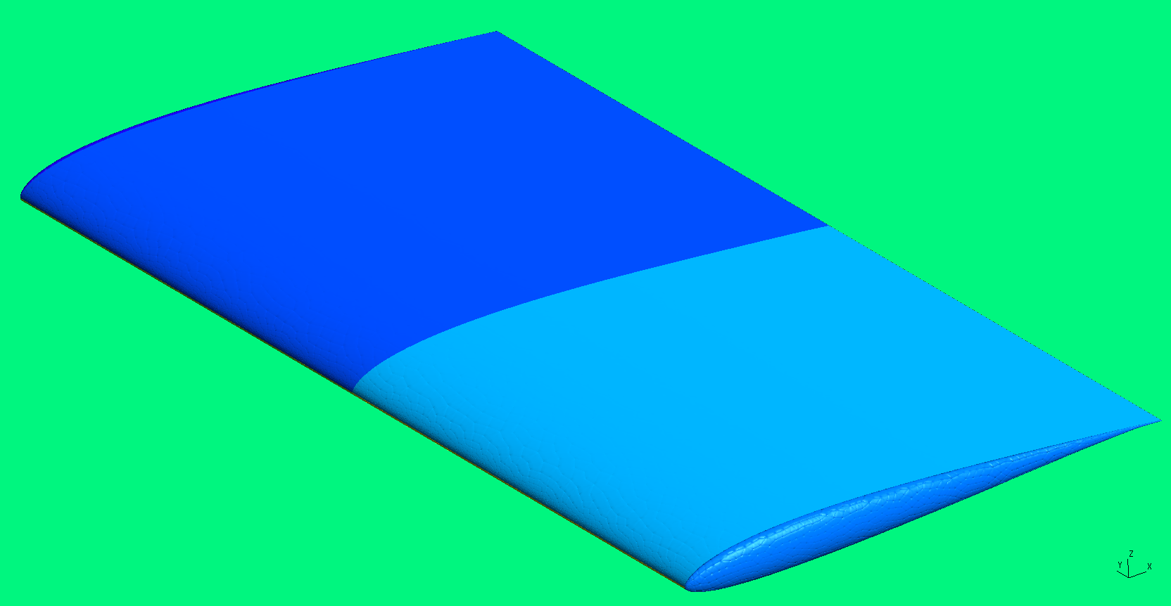
Again, we see that the surface is not plotted smoothly, since GMSH assumes we generated the mesh with equispaced points. If we make another mesh, this time with equispaced node locations, we will see a nice smooth surface: