This is a script to analyze the trajectories of supercooled water.

Requirements

• VMD 1.9.1 (or later) is required because the catdcd program is used.
• GROMACS 4.6.7 is required because the trjconv program is used. More recent versions of GROMACS are also probably okay.
• The following Python packages are needed: numpy, scipy, matplotlib, mdtraj, networkx, openmm (The latter is only for the units package).

Usage

Before running, make sure the paths to catdcd and trjconv are properly set in the script and you can run them on the command line without errors (i.e. no missing .so files or other issues with the environment.)

Run the analysis script as (assuming the codes are located in $HOME/src/supercool-analysis:

~/src/supercool-analysis/analyze.py (options) waterbox.pdb dynamics_0.dcd dynamics_1.dcd dynamics.dcd

where the .dcd files are in chronological order. The trajectories are concatenated during the analysis.

The script first uses catdcd to convert the trajectory into a .trr file, then uses trjconv to produce two .xtc files, one of which is "unwrapped" (i.e. atoms can diffuse outside of the periodic box). It then computes various properties, such as the diffusion coefficient, density, local structure index, and global / molecular Q6 order parameters.

Running analyze.py -h shows the available command line options. In most cases the default should work. For trajectories below 200 K, adding a stride of 10 frames via --stride 10 should decrease processing times with minimal impact on accuracy.

The script will produce output files in an analysis_results subfolder of the working folder containing the following:

• traj_steps.xtc and traj_steps.txt contain the trajectory frames and frame numbers that were selected for analysis. The analyzed frames are equally spaced in time over the whole concatenated trajectory. By modifying the --resolution option you can choose whether to analyze more or fewer frames.
• density.txt contains the density of the selected trajectory frames in kg/m^3.
• ln_diff.txt contains the natural log of the diffusion coefficient in units of cm^2 s^-1 for each molecule at the selected trajectory frames. (water at room temperature has a diffusion coefficient of 2.3e-5 cm^2 s^-1).
• Q6g.txt, Q6.txt contain the average and per-molecule Q6 order parameter for the selected trajectory frames.
• LSI.txt contains the per-molecule local structure index for the selected trajectory frames.

Other properties for analysis can be easily implemented by following the existing structure in the analysis script.

By default, if the output files from a previous run exist, the script will attempt to read them and skip over computing that property if reading is successful. This is for ease of making tweaks to the visualization method; it wouldn't be very efficient to rerun the analysis every time we wanted to adjust the plotting. However, if you want to rerun the analysis using different command line options (or a longer trajectory) it is recommended to delete or move the analysis_results folder before proceeding.

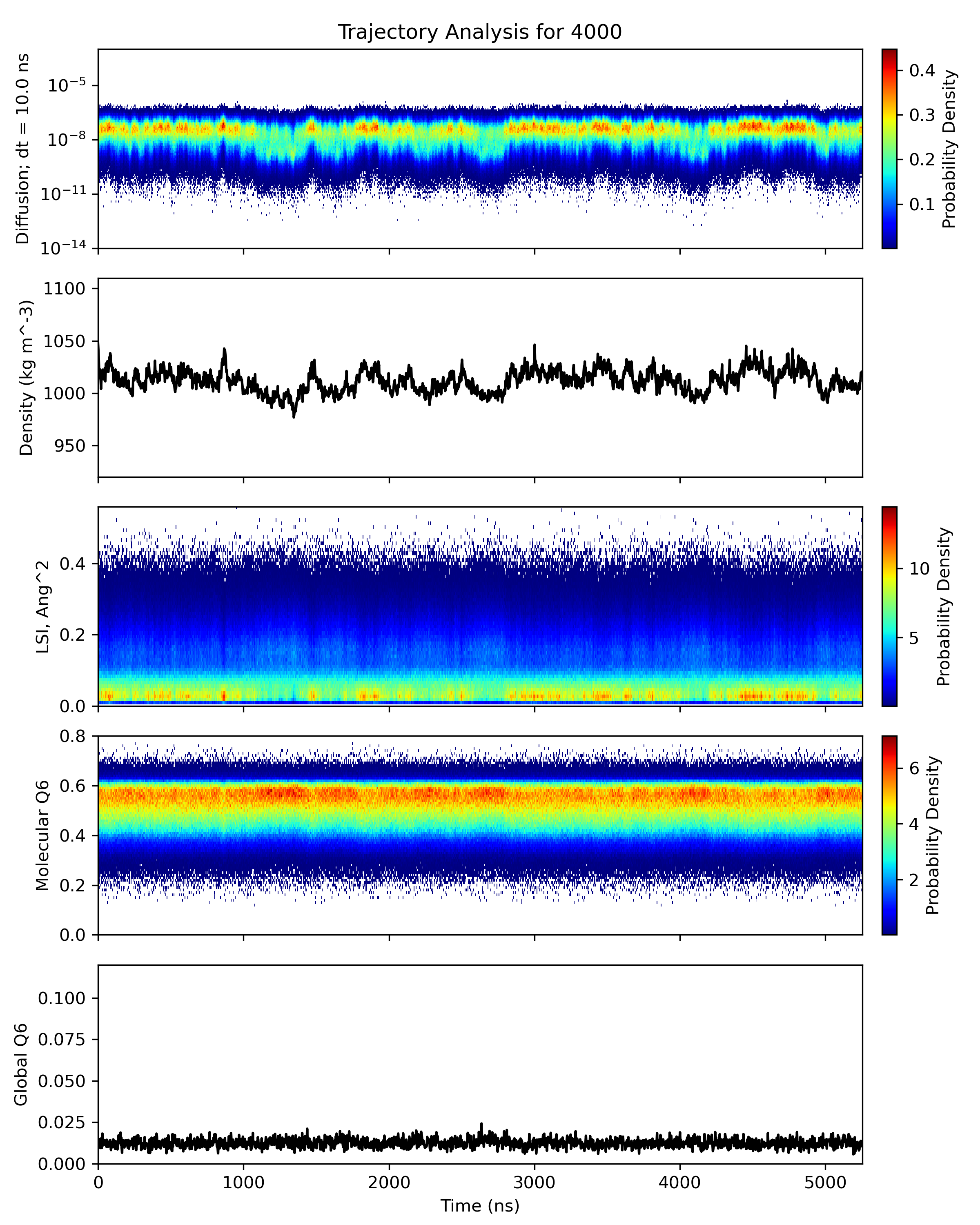
The script also produces plot.png which includes time series plots of the global and per-molecule properties.

Visualization

To visualize a per-molecule property, run VMD as:

<inside of the analysis_results folder>
vmd -e ~/src/supercool-analysis/watercolors.vmd -args ../waterbox.pdb traj_steps.xtc ln_diff.txt

(Here ln_diff.txt is used as an example but you should be able to visualize any of the per-molecule property text files.)

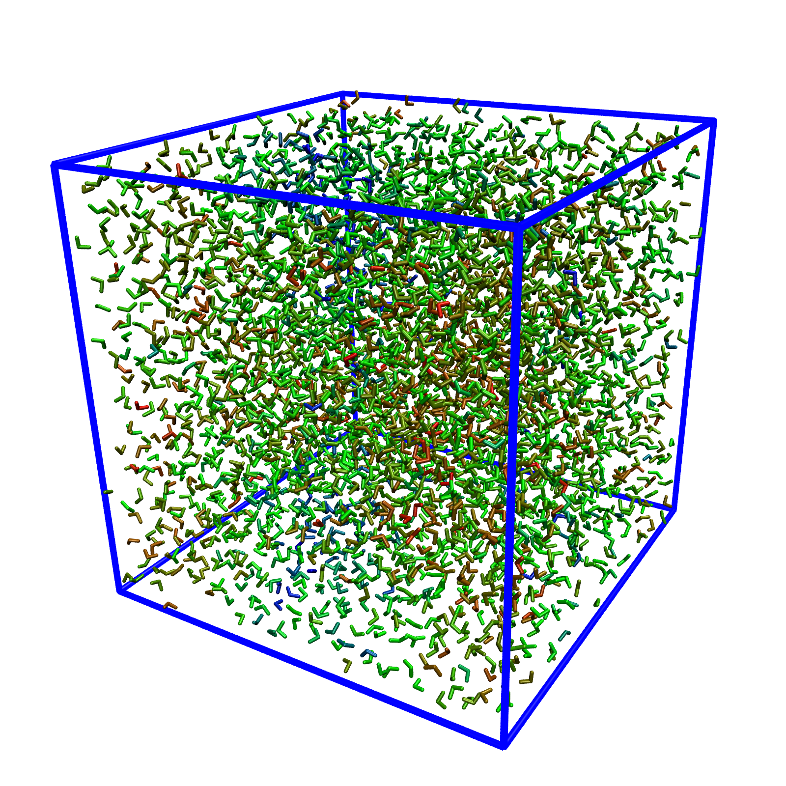
If it works properly, the property will be visualized as follows. You might want to change the representation to show the oxygens only (in Graphical Representations, change Licorice to VDW, set the atom selection to name O and set the sphere size of 0.5.) Increasing the trajectory smoothing window size could make things look less "jumpy", but my experience is don't increase it above 5 because VMD seems to get confused if the molecule being smoothed jumps across the boundary.

You can create a movie by selecting "Extensions -> Visualization -> Movie Maker" in VMD, setting "Movie Settings -> Trajectory", and disabling "Movie Settings -> Delete image files". I recommend making a subfolder analysis_results/frames to hold the outputs because a large number of files will be generated. VMD will automatically render the image files and then call a program to compress them into a movie. I prefer to ignore the VMD-generated movie and instead run ffmpeg manually as:

<inside of the analysis_result folder>
ffmpeg -r 30 -an -i frames/frame.%05d.ppm -vcodec h264 -b:v 8000k -pix_fmt yuv420p out.mp4

To do

• It would be nice to have some marginal histograms in plot.png.
• I would like to add a text label feature for the timestamp in the visualization.
• Being able to plot some correlations of pairs of per-molecule or global properties would be awesome.