🧠 pyEEGPlot

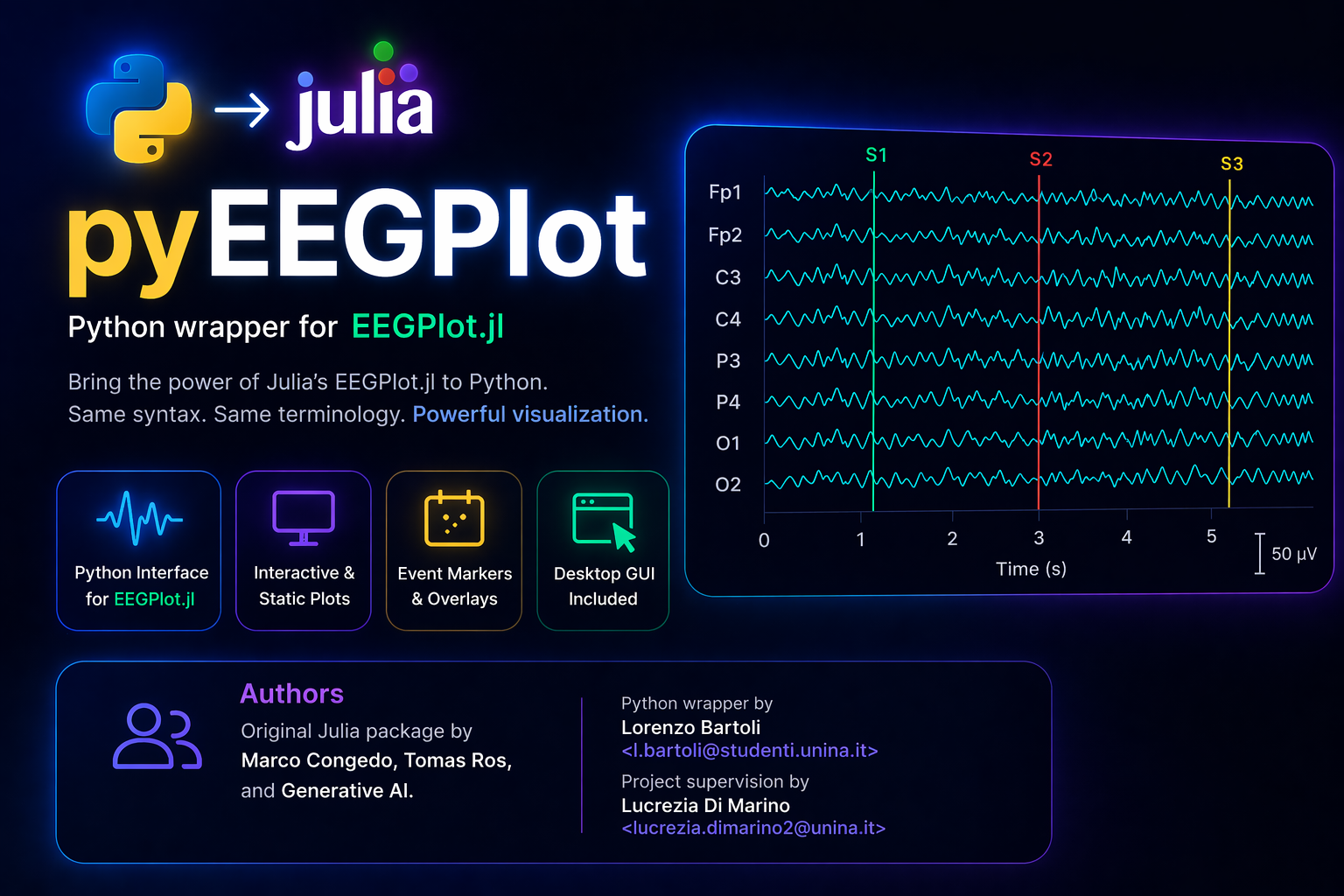
Bring the power of Julia's EEGPlot.jl to your Python workflow.

A Python wrapper for the Julia package EEGPlot.jl, designed to bring EEGPlot's visualization capabilities to Python while preserving the original function syntax and terminology as closely as possible.

Note: the first plot may take longer to appear because Julia compiles the required functions on first use. Subsequent plots are generated much faster.

⚙️ Features

• Python interface to EEGPlot.jl: Use the Julia plotting engine directly from Python.
• Static and Interactive Plots: Support both CairoMakie (static) and GLMakie (interactive) backends.
• Multiple Datasets: Plot EEG/ERP data with overlays and additional panels for artifacts or components.
• Event Markers: Visualize triggers and events as lines or blocks.
• Time Constant Consistency: Maintains a constant pixel-per-second scale regardless of sampling rate.
• Interactive Controls: Deep inspection of data via keyboard and mouse shortcuts (in interactive mode).
• GUI Support: Includes a desktop GUI to initialize the chosen backend, generate demo plot, and load EEG files for visualization.

📦 Installation

1. Install Julia

Before using pyEEGPlot, make sure that Julia is installed on your system and that the julia executable is available from your terminal or command prompt.

Install Julia from the official Julia installation page:

👉 https://julialang.org/install/

2. Install pyEEGPlot

You can install pyEEGPlot directly from PyPi:

pip install pyEEGPlot

Alternatively, you can install it from source:

git clone https://github.com/lore1907/pyEEGPlot.git
cd pyEEGPlot
pip install .

Or install it directly from GitHub:

# Or install it directly from Github
pip install git+https://github.com/lore1907/pyEEGPlot.git

After installing the Python package, run:

import pyEEGPlot as pyep
pyep.configure()

This step:

• creates an isolated Julia environment for pyEEGPlot,
• installs the required Julia dependencies,
• downloads EEGPlot.jl from GitHub,
• precompiles the Julia packages.

Note: the first-time Julia setup may take significantly longer than a typical pure-Python package installation because it also installs and precompiles Julia dependencies.

Once configuration is complete, you can initialize a backend and create plots normally.

🖥 Backend Initialization

pyEEGPlot provides explicit backend initialization. Two backends are supported:

• GLMakie for interactive plots
• CairoMakie for static plots and image export

Backend initialization is performed explicitly so that the plotting environment is configured in a predictable way before any figure is created. During this step, pyEEGPlot also performs a backend-specific warm-up procedure to reduce latency when generating the first actual plot.

In general:

• use GLMakie when you want to inspect signals interactively,
• use CairoMakie when you want fast static rendering or save plots as images.

Using init_plotting()

Before creating plots, you can explicitly initialize the desired backend with:

import pyEEGPlot as pyep
pyep.init_plotting(backend="static", do_warmup=False) 
#or
pyep.init_plotting(backend="dynamic", do_warmup=True)

The function allows you to:

• select the plotting backend explicitly,
• perform backend initialization before creating a figure,
• optionally run a warm-up step to reduce latency on the first real plot.

🧭 Two Ways to Use pyEEGPlot

pyEEGPlot can be used in two complementary ways:

1. Desktop GUI workflow

The GUI is intended for the most common visualization tasks and quick inspection of EEG files.

Use the GUI when you want to:

• initialize the selected backend,
• generate and display a demo plot,
• load EEG data from supported files (currently .edf and .txt),
• configure basic plotting options such as figure size and sampling rate,
• enable or disable event marker visualization, when available,
• save plots as .png when using the static backend.

2. Python API workflow

The Python API is intended for advanced and fully customizable use.

Use the Python API when you want to:

• work directly in scripts or notebooks,
• integrate plotting into an existing EEG analysis pipeline,
• use advanced keyword arguments from EEGPlot.jl,
• plot overlays, projections, lower panels, or auxiliary signals,
• combine pyEEGPlot with NumPy, SciPy, scikit-learn, MNE, or custom preprocessing steps.

In general, the GUI covers common usage, while the Python API provides the full flexibility of the wrapper.

🪟 Desktop GUI

To launch the GUI, run:

python -m pyEEGPlot.eeg_gui

Note: GUI startup and backend initialization may take some time on first use, especially when Julia compilation is required.

GUI limitations

The GUI is currently designed for common use cases and basic file visualization.

Some advanced EEGPlot.jl features are not implemented in the GUI yet, including for example:

• overlays and projections,
• additional lower panels (Y, Y_size),
• advanced combinations of keyword arguments.

For these cases, use the Python API directly.

Supported File Formats

The GUI currently supports loading:

• .edf files,
• .txt files.

When loading data from supported files, pyEEGPlot extracts the signal matrix and, when possible, any event-related information needed for event marker visualization. Depending on the file content and available metadata, some plotting options may or may not be enabled.

Event Visualization

When event or trigger information is available, pyEEGPlot can display temporal markers on the EEG timeline.

These markers can be enabled or disabled from the GUI. At the moment, event durations are not represented. Events are currently rendered as fixed-width onset markers rather than variable-duration intervals.

Event visualization is especially useful for:

• stimulus onsets,
• experimental triggers,
• time-locked inspection of EEG activity.

🚀 Quick Start with Python API

The following examples mirror the EEGPlot.jl Quick Start and illustrate common usage patterns in Python.

Static Plot

Static plots are generated with the CairoMakie static backend. This backend is suitable for fast, non-interactive visualization and for exporting images of the signal. Here are two quick examples:

import numpy as np
import pyEEGPlot as pyep

# One-time setup on a new machine
# pyep.configure()

pyep.init_plotting(backend="static", do_warmup=False)

X = np.random.randn(512, 4)
sr = 128
labels = ["Fp1", "Fp2", "C3", "C4"]

fig = pyep.eegplot(X, sr, labels, fig_size=(800, 400))

Here is a second example using Julia-side data loading:

import numpy as np
from pyEEGPlot import eegplot
from julia import Eegle, CairoMakie

# Activate static backend
CairoMakie.activate_()

# Read example EEG data using Eegle.jl
X = Eegle.readASCII(Eegle.EXAMPLE_Normative_1)
sr = 128
sensors = Eegle.readSensors(Eegle.EXAMPLE_Normative_1_sensors)

# Plot EEG
eegplot(X, sr, sensors, fig_size=(814, 450))

In this example:

• X contains the EEG data matrix,
• sr is the sampling rate,
• sensors contains sensor location information,
• fig_size controls the output figure size in pixels.

Multiple Datasets (PCA Example)

pyEEGPlot also supports visualization of additional signals derived from the original EEG data. This is useful, for example, when displaying PCA component scores, projections, artifact-related signals, or other auxiliary time series alongside the main EEG plot.

from pyEEGPlot import eegplot
from julia import Eegle, CairoMakie, LinearAlgebra, Statistics


# Read data
X = Eegle.readASCII(Eegle.EXAMPLE_Normative_1)
sr = 128
sensors = Eegle.readSensors(Eegle.EXAMPLE_Normative_1_sensors)


# Basic PCA projection using Julia's LinearAlgebra
# (Note: In Python you could also use scikit-learn or numpy)
cov = Statistics.cov(X)
vals, vecs = LinearAlgebra.eigen(cov)
u = vecs[:, -1:] # Principal component axis


y = X @ u        # Component scores (T x 1)
P = y @ u.T      # Projection (T x N)


eegplot(X, sr, sensors,
        fig_size=(814, 614),
        overlay=P,
        Y=y,
        Y_size=0.1)

In this example:

• overlay=P adds a channel-wise projection over the main EEG traces,
• Y=y displays an additional lower panel containing the component scores,
• Y_size=0.1 sets the relative height of the additional panel.

This mechanism is particularly useful when comparing original signals with model-based reconstructions or low-dimensional summaries.

📖 Documentation

For more examples and detailed information on arguments, keyword arguments, and interactive controls, please refer to the official EEGPlot.jl documentation:

👉 EEGPlot.jl Documentation

✍️ Authors

Original Julia package by Marco Congedo, Tomas Ros, and Generative AI.
Python wrapper by Lorenzo Bartoli l.bartoli@studenti.unina.it.
Project supervision by Lucrezia Di Marino lucrezia.dimarino2@unina.it.

📄 License

This project is released under the MIT License.