R package

Versión en español

R package

The R package monitoreo calls, with reticulate, the functions of the Python package: it computes exactly the same as the QGIS plugin and the MCP server. It returns data.frames, GeoTIFF paths for terra and, with rgee, Earth Engine images.

The options (regions, periods, metrics, filters) are explained in Concepts. The examples on this page are real and use the Sierra Nevada National Park (WDPA ID 389011).

Installation

1. The Python of MonitorEO. The simplest is the conda environment of Getting started (and earthengine authenticate, only to use your Earth Engine account).

2. The R package, from GitHub:

   install.packages(c("remotes", "reticulate", "ggplot2", "sf", "terra", "leaflet"))
   remotes::install_github("monitoreo-obsnev/monitoreo", subdir = "r/monitoreo")

   For a specific version (the one cited with its DOI), add ref = "v0.3.2"; from a clone of the repository, install.packages("r/monitoreo", repos = NULL, type = "source").

3. Tell R which Python to use, before loading the package or in ~/.Renviron:

   Sys.setenv(RETICULATE_PYTHON = "/Users/ana/miniforge3/envs/monitoreo/bin/python")
   # Windows: "C:/Users/ana/miniforge3/envs/monitoreo/python.exe"

   If you already use rgee with its own Python, you can install the Python package in it with mo_install().

1. Connect

library(monitoreo)
mo_init()                        # without the EE_PROJECT variable: the shared account of MonitorEO
# mo_init("my-ee-project")       # or your account and your project (or mo_init() with EE_PROJECT); mo_init(""): the shared one
mo_eecu()                       # your EECUs of this month; with your project, mo_eecu("Contributor") if that is its tier

With the shared account they are your research EECUs (25 EECU-h per month, for research only): if less than 10 % is left, mo_init() and the functions that compute give a warning() (once a month) asking you to switch to your account, and when they run out the shared account does not compute until the next month (Concepts).

When loaded, the package shows the description and the acknowledgements of MonitorEO; mo_about("en") gives them in English.

2. Variables and regions

mo_variables(sensor = "Modis", text = "NDVI")[, c("ref", "variable", "sensor", "collection", "resolution_m")]

  ref variable sensor        collection resolution_m
1  25     NDVI  Modis MODIS/061/MOD13Q1          250
2  26     NDVI  Modis MODIS/061/MYD13Q1          250

mo_protected_areas("Doñana")[, c("SITE_ID", "NAME", "DESIG", "IUCN_CAT")]

    SITE_ID                 NAME                                          DESIG IUCN_CAT
1 555588792               Doñana Zona de Importancia Comunitaria ZIC (ZEPA/ZEC)       IV
2 555595662 Doñana Norte y Oeste Zona de Importancia Comunitaria ZIC (ZEPA/ZEC)       IV
3    389012               Doñana                                Parque Nacional       II
4    349268               Doñana                                 Parque Natural        V
...

Regions are built with functions:

sn <- mo_wdpa(389011)                          # one or several protected areas: mo_wdpa(c(389011, 389012))
mo_ecoregion(793)                              # ecoregion by ID, or mo_ecoregion(lon = -3.3, lat = 37.1)
mo_bbox(-3.6, 36.9, -2.6, 37.3)                # west, south, east, north
mo_point(-3.42, 37.13, buffer = 1500)          # circle of 1.5 km
zones <- mo_sf(sf::st_read("zonas.gpkg"), "nombre")   # any sf object of polygons; one series per polygon

3. Time series

ts <- mo_time_series(sn, "NDVI", "Sentinel-2", "2022-01-01", "2023-12-31", step = "monthly")
head(ts, 3)

        date n_images n_pixels        region     value
1 2022-01-01       30   346520 Sierra Nevada 0.3536522
2 2022-02-01       29   298880 Sierra Nevada 0.4035685
3 2022-03-01       31   224912 Sierra Nevada 0.2237470

It is a data.frame with Date dates and the attributes title, unit and scale (the pixel used, here 50 m).

mo_plot(ts)                                    # ggplot2: you can keep adding layers
write.csv(ts, "ndvi.csv", row.names = FALSE)   # or mo_time_series(..., csv = "ndvi.csv")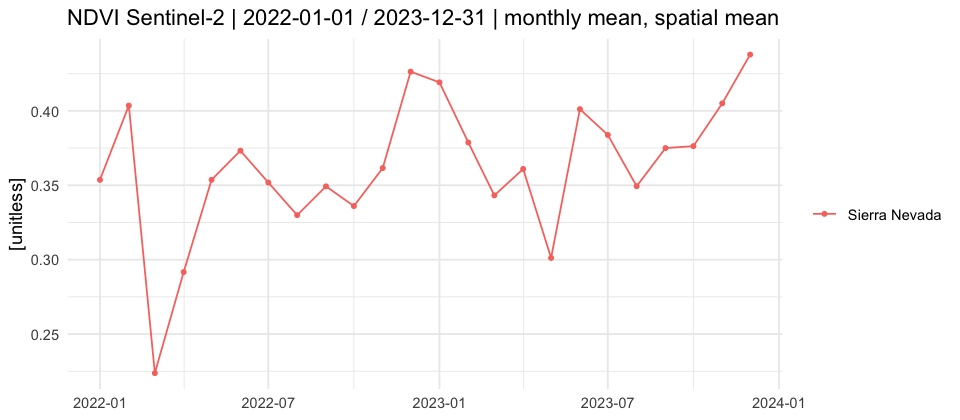

More examples:

mo_time_series(sn, "LST", "Landsat", "2015-01-01", "2023-12-31", step = "annual", metric = "max")
mo_time_series(zones, "NDVI", "Sentinel-2", "2023-01-01", "2023-12-31", season = c("06-01", "09-30"))
mo_time_series(sn, "NDSI", "Modis", "2022-10-01", "2023-06-30", step = "16-day", quality = list(snow = FALSE))

4. Maps

Earth Engine tiles in leaflet (over an orthoimage):

layer <- mo_map_layer(sn, "NDVI", "Sentinel-2", "2023-06-01", "2023-08-31")
mo_leaflet(layer)

With rgee, the Earth Engine image and its colour ramp:

x <- mo_image(sn, "LST", "Modis", "2023-06-01", "2023-08-31", metric = "mean")
rgee::Map$centerObject(x$image, 10)
rgee::Map$addLayer(x$image, x$vis, x$name)

Statistics of a map in each polygon:

mo_region_stats(sn, "LST", "Modis", "2023-06-01", "2023-08-31", metric = "mean")
#          region     mean      std      min       p5      p50      p95      max n_pixels
# 1 Sierra Nevada 32.20741 1.976974 27.26778 29.40603 32.08767 34.90077 40.85588     1051

As GeoTIFF, for terra (small or medium regions; for large ones, use mo_export_image() to Google Drive):

f <- mo_download_image(mo_point(-3.42, 37.13, 1500), "NDVI", "Sentinel-2", "2023-01-01", "2023-12-31",
                       path = "ndvi_p95.tif", metric = "p95")
terra::plot(terra::rast(f$file))

5. Trends

The trend of the NDVI of each month from 2005 to 2024 (MODIS):

tr <- mo_trend_table(sn, "NDVI", "Modis", "2005-01-01", "2024-12-31", step = "monthly")
tr[, c("label", "n", "tau", "p_value", "significant", "slope")]

       label  n         tau     p_value significant         slope
1    January 20 -0.06315789 0.697031003       FALSE -0.0002659812
2   February 20  0.07368421 0.649670504       FALSE  0.0006624354
3      March 20  0.25263158 0.119393190       FALSE  0.0014753512
4      April 20  0.04210526 0.795207612       FALSE  0.0003653394
5        May 20  0.10526316 0.516412268       FALSE  0.0008568967
6       June 20  0.18947368 0.242809091       FALSE  0.0011871008
7       July 20  0.17894737 0.269981282       FALSE  0.0013375445
8     August 20  0.45263158 0.005267412        TRUE  0.0018529123
9  September 20  0.36842105 0.023140931        TRUE  0.0019901468
10   October 20  0.13684211 0.398920137       FALSE  0.0010093510
11  November 20  0.12631579 0.436178362       FALSE  0.0011457025
12  December 20  0.10526316 0.516412268       FALSE  0.0004527001

Only August and September have a significant trend (p < 0.05): about +0.002 NDVI units per year. attr(tr, "yearly") has the values of each year and mo_trend_table(..., chart = "trends.png") draws the chart of each month with its Sen line.

In each pixel, as GeoTIFF with the bands slope, tau, z, p_value, intercept and n:

f <- mo_download_trend(sn, "NDVI", "Modis", "2005-01-01", "2024-12-31", path = "trend.tif")   # step = "annual"
r <- terra::rast(f$file)
r

class       : SpatRaster
size        : 121, 315, 6  (nrow, ncol, nlyr)
resolution  : 250, 250  (x, y)
coord. ref. : WGS 84 / UTM zone 30N (EPSG:32630)
names       :   slope, tau,         z, p_value, intercept,  n

slope <- terra::ifel(r$p_value < 0.05, r$slope, NA)      # only the significant trend
terra::plot(slope, col = hcl.colors(11, "RdYlGn"), range = c(-0.005, 0.005))

For one month: step = "monthly", part = 8 (August). The tile map: mo_leaflet(mo_trend_map(...)).

6. Compare two periods

cmp <- mo_compare_series(sn, "NDVI", "Modis", "2005-01-01", "2009-12-31",    # reference
                         "2020-01-01", "2024-12-31")                         # other period
head(cmp[, c("label", "reference", "other", "difference")], 3)

     label reference     other    difference
1  January 0.4954321 0.4952818 -0.0001502843
2 February 0.4680880 0.4829461  0.0148581591
3    March 0.4335899 0.4606720  0.0270820311

The map of the difference: mo_compare_map() (tiles) or mo_download_comparison() (GeoTIFF with the bands difference, reference and other).

7. Burn severity

s <- mo_burn_severity(mo_wdpa(389013), "2023-05-15", "2023-08-14", "2023-09-15", "2023-11-30",
                      path = "severity.tif")          # Sentinel-2; sensor = "Landsat" for earlier fires
s[s$class >= 1, c("label", "ha")]                     # hectares of each severity class
terra::plot(terra::rast(attr(s, "file"))$severity)
r <- mo_burn_severity(mo_wdpa(389013), "2023-05-15", "2023-08-14", "2023-09-15", "2023-11-30",
                      index = "RBR", path = "rbr.tif")  # the RBR: mean, median, p10, p90, min, max and ha

8. Exports and recipes

task <- mo_export_image(sn, "NDVI", "Sentinel-2", "2023-01-01", "2023-12-31", resolution = 10, folder = "MonitorEO")
mo_task_status(task$operation)

mo_download_variables("recipe.yaml", "zone.gpkg", "variables", dry_run = TRUE)   # recipe: see the Python package page
mo_download_variables("recipe.yaml", "zone.gpkg", "variables")
terra::rast(list.files("variables", "\\.tif$", full.names = TRUE))

The recipe can be a YAML or an R list (yaml::read_yaml()); its format is in Python package.

Functions

Function	What it does
mo_init(), mo_install(), mo_about()	Connect, install the Python package, description and acknowledgements
mo_eecu()	Your Earth Engine EECUs spent this month (research EECUs with the shared account)
mo_variables(), mo_describe()	Variables of the catalog
mo_protected_areas()	Search WDPA protected areas
mo_wdpa(), mo_ecoregion(), mo_bbox(), mo_point(), mo_geojson(), mo_sf()	Regions
mo_time_series(), mo_plot()	Time series and its chart
mo_map_layer(), mo_leaflet(), mo_image()	Maps: tiles, leaflet and rgee
mo_region_stats()	Statistics of a map by polygon
mo_download_image(), mo_download_variables()	GeoTIFF on the computer
mo_trend_table(), mo_trend_map(), mo_download_trend()	Seasonal trends
mo_compare_series(), mo_compare_map(), mo_download_comparison()	Comparison of periods
mo_burn_severity()	Burn severity (dNBR, USGS classes; or the RBR with index = "RBR")
mo_export_image(), mo_export_time_series(), mo_task_status()	Exports to Google Drive

The arguments are those of the functions of the same name of the Python package.