ML Grade Predictor

Marks Prediction Using Linear & Polynomial Regression — Built From Scratch

A machine learning project implementing regression algorithms from the ground up using only Python and NumPy — no high-level ML libraries such as scikit-learn. Developed as a demonstration of foundational understanding of statistical learning theory and numerical optimisation.

---

Table of Contents

1. Project Overview
2. Key Features
3. Mathematical Foundation
4. Model Architecture
5. Performance Metrics
6. Project Structure
7. Installation & Setup
8. How to Run
9. Results & Visualisations
10. Sample Output

---

Project Overview

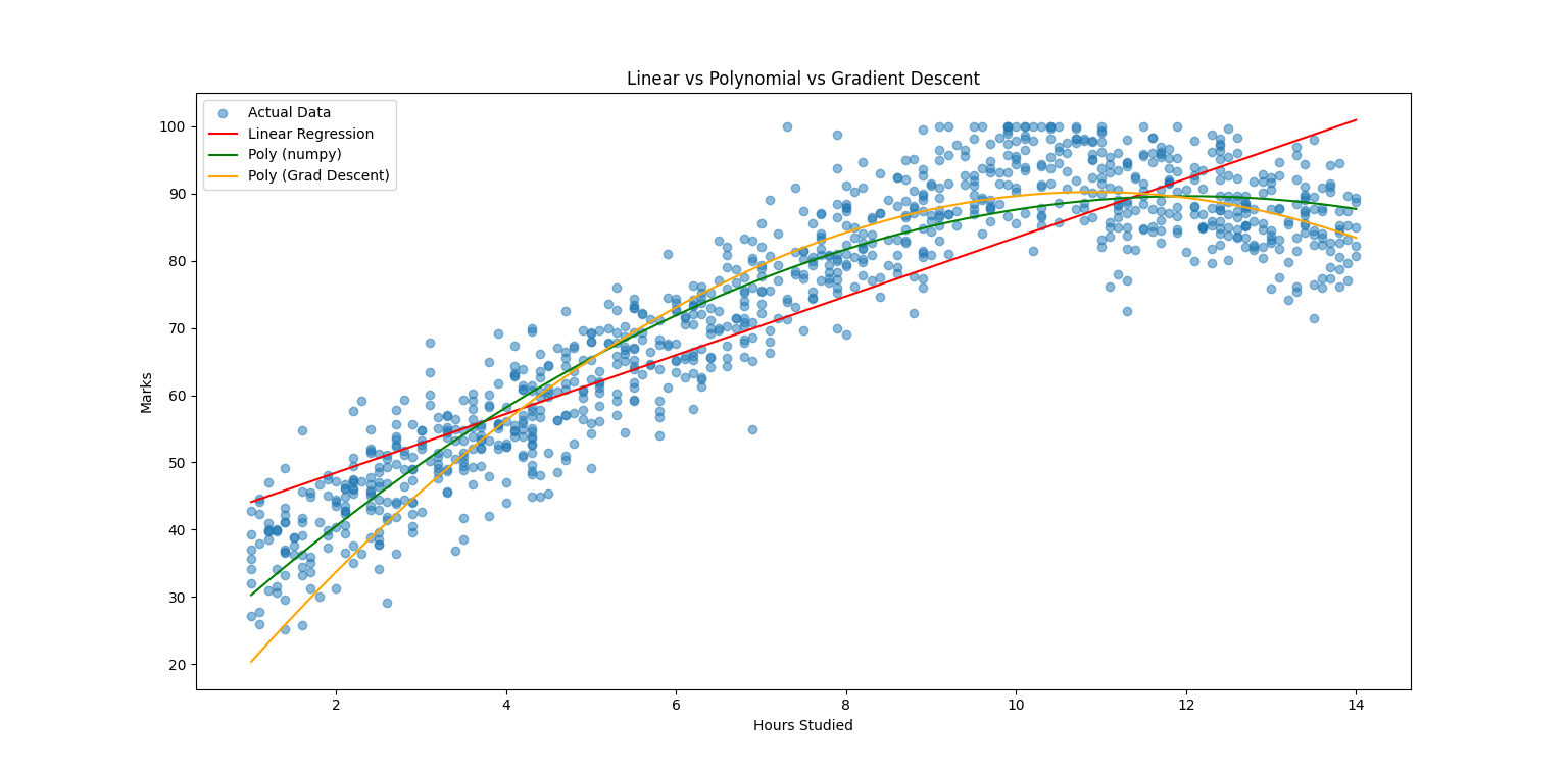
This project predicts student exam marks based on hours studied by training and comparing three regression models side-by-side:

Model	Method
Linear Regression	Closed-form analytical solution (Normal Equation)
Polynomial Regression (NumPy)	NumPy polyfit as a reference baseline
Polynomial Regression (Gradient Descent)	Iterative optimisation implemented entirely from scratch

The dataset contains 1,000+ student records spanning 1.0–14.0 study hours. An 80/20 train-test split is applied after random shuffling to ensure unbiased evaluation.

---

Key Features

• Three models in one script — direct side-by-side comparison of Linear Regression, NumPy Polynomial, and from-scratch Gradient Descent Polynomial
• Zero high-level ML dependencies — every algorithm is implemented manually; no scikit-learn or similar libraries
• Live training feedback — R² score is logged to the console every 10,000 epochs during gradient descent
• Interactive prediction — after training, the user can enter any value (1.0–13.9 hours) and receive predictions from all three models simultaneously
• Overfitting diagnostics — explicit train vs. test R² comparison printed after training
• Learning curve plot — R² score tracked against epoch count to visualise model convergence

---

Mathematical Foundation

All mathematical operations are implemented from scratch without relying on library abstractions.

Descriptive Statistics

Mean

$$\bar{x} = \frac{1}{n} \sum_{i=1}^{n} x_i$$

Median — computed via manual sorting and index selection for both even and odd-length arrays.

Variance & Standard Deviation

$$s^2 = \frac{\sum_{i=1}^{n}(x_i - \bar{x})^2}{n - 1} \qquad s = \sqrt{s^2}$$

---

Linear Regression (Closed Form)

Slope (m)

$$m = \frac{\sum_{i=1}^{n}(x_i - \bar{x})(y_i - \bar{y})}{\sum_{i=1}^{n}(x_i - \bar{x})^2}$$

Intercept (c)

$$c = \bar{y} - m\bar{x}$$

Prediction

$$\hat{y} = mx + c$$

---

Polynomial Regression (Degree 2)

$$\hat{y} = Ax^2 + Bx + C$$

---

Gradient Descent Optimisation

Coefficients A, B, C are initialised to zero and updated iteratively by minimising the Mean Squared Error loss:

$$\mathcal{L} = \frac{1}{n}\sum_{i=1}^{n}(\hat{y}_i - y_i)^2$$

Partial gradients:

$$\frac{\partial \mathcal{L}}{\partial A} = \frac{2}{n}\sum({\hat{y}_i - y_i}) \cdot x_i^2$$

$$\frac{\partial \mathcal{L}}{\partial B} = \frac{2}{n}\sum(\hat{y}_i - y_i) \cdot x_i$$

$$\frac{\partial \mathcal{L}}{\partial C} = \frac{2}{n}\sum(\hat{y}_i - y_i)$$

Update rule:

$$\theta \leftarrow \theta - \alpha \cdot \nabla_\theta \mathcal{L}$$

Hyperparameter	Value
Learning Rate (α)	1e-5
Epochs	150,000

---

Performance Metrics

R² (Coefficient of Determination)

$$R^2 = 1 - \frac{\sum(y_i - \hat{y}_i)^2}{\sum(y_i - \bar{y})^2}$$

Average Absolute Error (AAE)

$$\text{AAE} = \frac{1}{n}\sum_{i=1}^{n}|y_i - \hat{y}_i|$$

Average Percentage Error (APE)

$$\text{APE} = \frac{1}{n}\sum_{i=1}^{n}\frac{|y_i - \hat{y}_i|}{y_i} \times 100$$

---

Model Architecture

Input: Hours Studied (float, range 1.0 – 14.0)
        │
        ├─── Linear Regression ──────────── ŷ = mx + c
        │      └── Analytical closed-form solution
        │
        ├─── Polynomial Regression (NumPy)── ŷ = ax² + bx + c
        │      └── numpy.polyfit baseline
        │
        └─── Polynomial Regression (GD) ─── ŷ = Ax² + Bx + C
               └── Manual gradient descent (150,000 epochs)
                        │
                Output: Predicted Mark (0 – 100)

---

Project Structure

ML-Grade-Predictor/
│
├── ml_grade_predictor.py     # Main script — all models and visualisations
└── README.md                 # Project documentation

---

Installation & Setup

Ensure Python 3.x is installed, then install the two required libraries:

python -m pip install numpy==1.26.4 matplotlib==3.8.4

Windows users — if the above command does not work, try:

py -m pip install numpy==1.26.4 matplotlib==3.8.4

Dependencies summary:

Library	Version	Purpose
numpy	1.26.4	Array operations & polyfit baseline
matplotlib	3.8.4	Regression and learning curve plots

No other external dependencies are required.

---

How to Run

Navigate to the project directory and execute:

python ml_grade_predictor.py

Windows alternative: py ml_grade_predictor.py

What happens at runtime:

1. The dataset is shuffled and split 80/20 into training and test sets
2. All three models are trained; gradient descent logs progress every 10,000 epochs
3. Final R² scores and overfitting diagnostics are printed to the console
4. Two plots are displayed — regression curves and the learning curve
5. The user is prompted to enter hours studied and receives predictions from all three models
6. Average absolute error and average percentage error on the test set are printed

---

Results & Visualisations

Plot 1 — Regression Curves

Displays the raw scatter data alongside all three fitted curves, enabling direct visual comparison of how each model captures the underlying trend.

Plot 2 — Learning Curve (Gradient Descent)

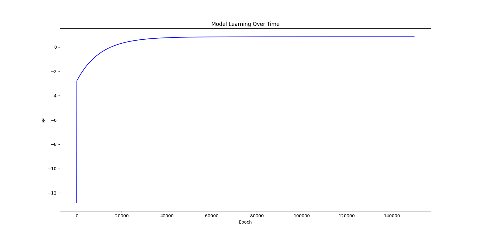
Tracks R² score against epoch number across 150,000 training iterations, illustrating the convergence behaviour of the gradient descent optimiser.

---

Sample Output

Epoch      0 | A:0.001 B:0.003 C:0.002 | Test R²:0.1234
Epoch  10000 | A:0.412 B:3.821 C:22.10 | Test R²:0.8901
Epoch 150000 | A:0.387 B:4.105 C:21.47 | Test R²:0.9312

--- Final R² Scores (full dataset) ---
Linear regression    : 0.9187
Poly (numpy)         : 0.9324
Poly (grad descent)  : 0.9312

--- Train vs Test R² (overfitting check) ---
Train R²: 0.9338
Test  R²: 0.9312

Enter Hours Studied: 7.5
Linear Prediction             : 68.43
Numpy Polynomial Prediction   : 69.81
Gradient Polynomial Prediction: 69.74

Avg abs error on test set : 4.21 marks
Avg % error on test set   : 5.38%

---

Note: Actual R² values and predictions will vary slightly between runs due to random shuffling of the dataset before the train-test split.