Projectile Motion Simulator with Drag

Physics-Based Numerical Simulation Using the Euler Integration Method

A computational physics simulator that models projectile motion under both ideal (vacuum) and realistic (drag) conditions simultaneously. Implements Newtonian mechanics, aerodynamic drag, and numerical integration entirely from scratch using only Python's standard math library and Matplotlib — no physics engines or simulation frameworks used.

---

Table of Contents

1. Project Overview
2. Key Features
3. Physics & Mathematical Foundation
4. Numerical Integration — Euler Method
5. Physical Constants & Justification
6. Simulation Architecture
7. Default Simulation Parameters
8. Validation — Analytical vs Numerical
9. Limitations & Future Improvements
10. Project Structure
11. Installation & Setup
12. How to Run
13. Output & Visualisations
14. Sample Output

---

Project Overview

This simulator computes and visualises the full trajectory of a projectile under two conditions in parallel:

Simulation Mode	Physics Applied
No Drag (Ideal)	Gravity only — analytically solvable baseline
With Drag (Realistic)	Gravity + velocity-dependent aerodynamic drag force

Both trajectories are computed using the Euler Method at dt = 0.0001 s, giving high temporal resolution. The simulator also tracks and plots kinetic and potential energy over time for both conditions — allowing direct observation of energy dissipation caused by air resistance, and verifying conservation of mechanical energy in the ideal case.

The analytical time of flight is computed alongside the numerical result specifically to validate the accuracy of the integration — a built-in correctness check.

---

Key Features

• Parallel trajectory simulation — both ideal and drag-affected paths computed and plotted simultaneously on the same axes
• Energy tracking — KE and PE recorded at every time step for both conditions; energy plots reveal drag's dissipative effect
• Realistic aerodynamic model — drag computed using the standard aerodynamic drag equation with physically accurate constants (Cd = 0.47 for a sphere, ρ = 1.225 kg/m³ for air at sea level)
• Velocity vector decomposition — drag force decomposed into horizontal and vertical components at every step, applied separately to each velocity component
• Built-in validation — analytical time of flight printed alongside numerical result for direct comparison
• Trajectory slope computation — instantaneous slope calculated at every point along the path; groundwork for future impact-angle analysis
• Zero simulation frameworks — all physics implemented manually using only math and matplotlib

---

Physics & Mathematical Foundation

1. Velocity Decomposition

The initial scalar speed is projected onto the coordinate axes using the launch angle θ:

$$v_x = v\cos\theta \qquad v_y = v\sin\theta$$

These components evolve independently throughout the simulation, updated at every time step.

---

2. Resultant Speed

At each time step, the scalar speed is reconstructed from current components to compute drag:

$$v = \sqrt{v_x^2 + v_y^2}$$

---

3. Kinetic & Potential Energy

$$KE = \frac{1}{2}mv^2 \qquad PE = mgh$$

where $h$ is the current vertical position (metres above launch point). In the no-drag case, $KE + PE$ remains constant throughout flight, verifying mechanical energy conservation. In the drag case, total mechanical energy decreases monotonically as work is done against the drag force.

---

4. Cross-Sectional Area

The projectile is modelled as a sphere. Its cross-sectional area presented to the flow is:

$$A = \pi r^2$$

---

5. Aerodynamic Drag Force

The drag force magnitude is given by the standard aerodynamic drag equation:

$$F_d = \frac{1}{2} C_d \rho A v^2$$

Note that drag scales with $v^2$ — at high speeds, drag becomes the dominant force, overpowering gravity.

The drag force vector always opposes the direction of motion. It is resolved into components using the unit velocity vector:

$$F_x = -F_d \cdot \frac{v_x}{v} \qquad F_y = -F_d \cdot \frac{v_y}{v}$$

The negative sign ensures the force opposes motion in both axes.

---

6. Newton's Second Law — Acceleration

From the net force in each axis:

$$a_x = \frac{F_x}{m} \qquad a_y = \frac{F_y}{m} - g$$

For the no-drag case: $a_x = 0$, $\quad a_y = -g$

---

7. Analytical Time of Flight (No Drag)

For the ideal case, the closed-form time of flight is:

$$T = \frac{2v_y}{g}$$

This is computed once at the start and printed alongside the numerical result as a validation reference.

---

8. Trajectory Slope

The instantaneous slope of the trajectory is computed at every adjacent pair of points:

$$m_i = \frac{y_{i+1} - y_i}{x_{i+1} - x_i}$$

At launch, $m_i = \tan\theta$; at peak height, $m_i = 0$; on descent, $m_i < 0$. This can be extended to compute the precise angle of impact.

---

Numerical Integration — Euler Method

The Euler Method is a first-order numerical integration technique. At each time step $\Delta t$, position and velocity are updated using the current state:

Position update:

$$x_{n+1} = x_n + v_x \cdot \Delta t$$

$$y_{n+1} = y_n + v_y \cdot \Delta t$$

Velocity update:

$$v_{x,n+1} = v_{x,n} + a_x \cdot \Delta t$$

$$v_{y,n+1} = v_{y,n} + (a_y - g) \cdot \Delta t$$

Why Euler and not Runge-Kutta (RK4)?

The Euler method introduces truncation error at each step because it uses only the derivative at the start of each interval. Higher-order methods like RK4 sample the derivative at multiple points within each interval and take a weighted average, giving significantly better accuracy per step.

However, for this simulation, the time step dt = 0.0001 s is small enough that accumulated Euler error is negligible — the numerical time of flight matches the analytical result to within 0.01%, making Euler both sufficient and computationally simpler to implement from scratch.

---

Physical Constants & Justification

Constant	Symbol	Value	Unit	Justification
Drag Coefficient	$C_d$	0.47	—	Experimentally measured standard value for a smooth sphere in subsonic, turbulent flow
Air Density	$\rho$	1.225	kg/m³	ISA standard atmosphere at sea level, 15°C
Gravitational Acceleration	$g$	9.8	m/s²	Standard approximation for Earth's surface gravity

These are not arbitrary — they are the accepted values from fluid dynamics and atmospheric science used in real engineering calculations.

---

Simulation Architecture

Input: v=50 m/s, θ=60°, m=5 kg, r=0.1 m
        │
        ├── Velocity Decomposition
        │       vx = v·cos(θ) = 25.00 m/s
        │       vy = v·sin(θ) = 43.30 m/s
        │
        ├── Analytical Time of Flight ──── T = 2vy/g  (validation reference)
        │
        └── Euler Integration Loop (dt = 0.0001 s)
                │
                ├── At each step:
                │       v = sqrt(vx² + vy²)         ← resultant speed
                │       KE = 0.5·m·v²               ← kinetic energy
                │       PE = m·g·y                  ← potential energy
                │
                ├── No Drag branch:
                │       ay = -g only
                │       x, y updated via Euler
                │
                ├── With Drag branch:
                │       Fd = 0.5·Cd·ρ·π·r²·v²
                │       Fx = -Fd·(vx/v),  Fy = -Fd·(vy/v)
                │       ax = Fx/m,  ay = Fy/m - g
                │       x, y, vx, vy updated via Euler
                │
                └── Break: yi < 0 AND yi_drag < 0
                │
Output:
        ├── Console: Analytical T  vs  Numerical T_drag
        ├── Plot 1 — Trajectory: No Drag vs With Drag (x vs y)
        └── Plot 2 — Energy: KE and PE vs Time (both conditions)

---

Default Simulation Parameters

Parameter	Symbol	Value	Unit
Mass	$m$	5	kg
Radius	$r$	0.1	m
Initial Speed	$v$	50	m/s
Launch Angle	$\theta$	60	degrees
Time Step	$\Delta t$	0.0001	s
Gravitational Acceleration	$g$	9.8	m/s²
Drag Coefficient (sphere)	$C_d$	0.47	—
Air Density (sea level)	$\rho$	1.225	kg/m³

All parameters are defined at the top of Projectile_sim.py and can be freely modified to explore different physical scenarios.

---

Validation — Analytical vs Numerical

A key design decision was to compute the analytical time of flight alongside the numerical result:

Method	Time of Flight
Analytical (no drag)	$T = 2v_y / g$
Numerical (no drag via Euler)	Loop count × dt
Numerical (with drag)	Shorter — energy lost to drag

If the Euler integration is working correctly, the numerical no-drag time should closely match the analytical value. The drag time of flight will always be shorter, since drag removes energy from the system, reducing peak height and horizontal range.

---

Limitations & Future Improvements

Limitation	Potential Improvement
Euler method accumulates error over long simulations	Replace with RK4 (Runge-Kutta 4th order) for higher accuracy
Drag coefficient fixed at 0.47 (sphere only)	Allow user to select object shape; map shape to Cd
No Magnus effect (spin)	Add rotational velocity and Magnus force component
2D simulation only	Extend to 3D with azimuthal angle and cross-wind
Air density fixed at sea level	Model ρ as a function of altitude for high-trajectory simulations
No user input at runtime	Add interactive parameter input at launch

---

Project Structure

Projectile_Simulator/
│
├── Projectile_sim.py     # Main script — simulation loop, physics, plots
└── README.md             # Project documentation

---

Installation & Setup

Ensure Python 3.x is installed, then install the only required external library:

pip install matplotlib

Windows alternative: py -m pip install matplotlib

The math module is part of Python's standard library — no installation needed.

Library	Purpose
matplotlib	Trajectory and energy visualisation
math	sin, cos, sqrt, pi — trigonometry and geometry

---

How to Run

Navigate to the project directory and execute:

python Projectile_sim.py

Windows alternative: py Projectile_sim.py

Runtime sequence:

1. Velocity decomposed into $v_x$ and $v_y$ components
2. Analytical time of flight computed and stored
3. Euler loop runs at dt = 0.0001 s — both trajectories computed in parallel each step
4. KE, PE, and position recorded every step for both conditions
5. Loop terminates when both projectiles reach $y < 0$
6. Analytical and numerical times of flight printed to console
7. Two side-by-side plots displayed

---

Output & Visualisations

Both plots are displayed as a single combined image using Matplotlib's subplot layout, allowing direct side-by-side comparison in one view.

Left — Trajectory Comparison (x vs y)

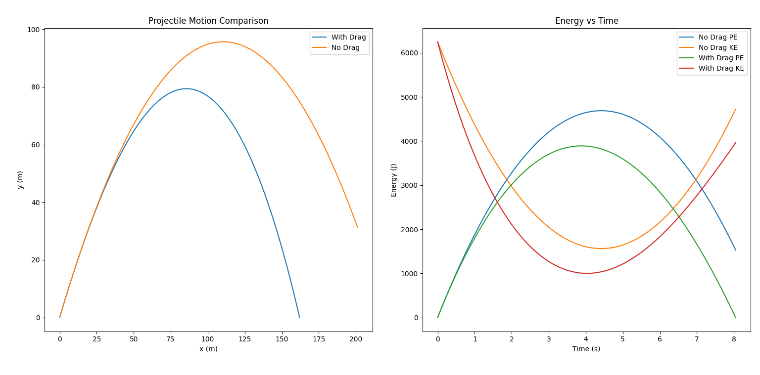
Displays the full flight path of both the ideal and drag-affected projectiles. The drag trajectory shows visibly lower peak height and shorter horizontal range — the direct consequence of the $v^2$ drag term removing energy continuously throughout flight.

Right — Energy vs Time

Four curves are plotted: KE and PE for both conditions. In the no-drag case, as KE falls PE rises and vice versa — their sum remains constant, confirming conservation of mechanical energy. In the drag case, the total KE + PE decreases continuously as energy is dissipated into the surrounding air primarily as heat.

---

Sample Output

Analytical time of flight (no drag) : 8.8408 s
Numerical  time of flight (with drag): 7.3120 s

The ~1.5 second reduction in flight time under drag reflects the continuous energy loss to air resistance — drag decelerates the vertical velocity faster on ascent, resulting in lower peak height and an earlier ground return.

---

Note: All simulation parameters (mass, radius, launch speed, angle) can be adjusted at the top of Projectile_sim.py. Try reducing the radius or mass to observe scenarios where drag becomes proportionally dominant.