Dynamic_and_stochastic_programming

Notes and programs from Platzi's Dynamic and stochastic programming with Python course

Index

[TOCM]

[TOC]

1. First Module Introduction
   1. class 1 course objectives
2. Second Module Dynamic Programming
   1. Class 2 Introduction to Dynamic programming
      • Richard Bellman
      • Memoization
   2. Class 3 Fibonacci numbers
3. Third Module Random Walk
   1. Class 4 What is Random Walk?
      • Brownian Motion
      • Quantum Cloud Sculpture
      • External links for random walk
   2. Class 5 Drunkard's Walk
4. Fourth Module Stochastic Programs
   1. Class 8 Introduction to Stochastic Programming
      • Deterministic vs Stochastic programming
      • Examples
   2. Class 9 Probabilities calculation
      • Probabilities
   3. Class 12 Statistical inference
      • Law of the large numbers
      • Gambler's fallacy
   4. Class 13 Mean
   5. Class 14 Variance and Standard Deviation
      • Variance
      • Standard-Deviation
   6. Class 15 Normal Distribution
      • Empiric Rule
   7. Class 16 What are Montecarlo Simulations
5. Fourth Module Sampling and Confidence Interval
   1. Class 20 Sampling
   2. Class 21 Central Limit Theorem
   3. Class 22 Linear Regresion
6. Fifth Module Conclusions
   1. Class 23 Conclusions

First Module Introduction

class 1 course objectives

• Learn when to use Dynamic programming and it's benefits.

• Understand the difference between stochastic and deterministic programming.

• Learn to use stochastic programming.

• Learn to create valid computational simulations.

Second Module Dynamic Programming

class 2 Introduction to Dynamic Programming

Richard Bellman

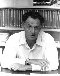
Richard Bellman introduced Dynamic Programming

Born in 1920 and died in 1984.

• Won the John Von Neumann Theory Prize in 1976.

• Studied mathematics at the Brooklyn College in 1941.

• He studied at the University of Wisconsin.

• Introduced Dynamic programming in the 1950s

"The name 'Dynamic programming' was chosen to hide from governmental sponsors 'the fact that I was really doing mathematics... [the phrase dynamic programming] was something not even a Congressman could object to.'" Introduction to Computation and Programming Using Python, With application to Understanding Data - John V. Guttag

Dynamic Programming == Mathematics

• Optimal Substructure: A global optimal solution can be found using local optimal sub-problems.

• Spliced problems: An optimal solution that can solve the same problem in different occasions.

Memoization

• Memoization is a technique to save previous results so you don't have to do it again.

• Normally is used with a dictionary, the queries can be made in O(1).

• Changes time for memory space (It's faster but consumes more memory)

Class 3 Fibonacci numbers

Can be defined by:

$$ F_n = F_{n-1} + F_{n-2}$$

This is a recursive formula, it's easy to implement in code but it's very inefficient.

The calculation repeats itself more than once.

It's exponential O.

So how can we optimize this implementation, first we use the recursive implementation and adding memoization. This approach has to be much better than only recursive.

In the dynamic implementation, I used a try, except flow control. In the dynamic programming, file added the dictionary where you store the previous calculations. Now you can do really big calculations of Fibonacci numbers.

note Python has a limit for recursion. The error is maximum recursion depth.

So if you want to avoid this error, I imported the sys module, and setting a new recursion limit.

Third Module Random Walk

class 4 What is random walk?

• It is a kind of simulation that takes a random decision in a set of valid decisions.
• it is used in a lot of fields of knowledge, when the deterministic decision aren't valid, and you need randomness.

Brownian motion

When the microscopic where invented, people saw that the particles moves were random.

Einstein saw that the pollen motion was made by the individual water molecules, and modeled the motion.

the atomic motion is random.

You can't model this kind of motion in deterministic programming.

Not only at the microscopic level works the random walk.

The smoke can be simulated by this.

The merge of two galaxies can be simulated, using the gravity, and the behavior of each star and other inputs can model possibles outputs.

Our galaxy the Milky Way is on track to collide and merge with Andromeda.

Scientists are making models using random walk to simulate what can be the final result when this happens.

Not only in physics is used the random walk. In market simulations is used too.

Quantum Cloud Sculpture

There is a sculpture called Quantum Cloud Sculpture, is located in London, and is next to the O2 (an entertainment district in Greenwich at the southeast of London).

External links for Random Walk

PBS infinite series

Socratica

Class 5 drunkard's walk

is an algorithm for a simulation.

starts at (0,0) in a Cartesian plane where you can move right, left, up, and down with the same probability (25%).

We can generate a Hypothesis, What happens after 10 steps? Are we close or are we far? what happens after 100, 1000, 10000 steps? What happens if we do it in 3 dimensions or 4. What happens if the distribution of probability is not the same?

You can calculate the final distance with the Pythagoras theorem.

the idea of this program is generate three classes.

1. class drunkard named drunk.

2. class abstraction of coordinates called coordinate.

3. class Cartesian plane called field (only in a field you can walk like this haha).

I did all the three classes and made all the program, now if you run it, you can see how far your drunkard's has gone.

There are two classes of drunkard's Traditional drunkard's who is aleatory and Fallen drunkard's who is trying to go up in a hill.

Fourth Module Stochastic Programs

Class 8 Introduction to Stochastic programming

Deterministic vs Stochastic programming

• A program is deterministic when if you use the same input you get the same output.
• Deterministic programming is very important but not all problems can be solved with this method.
• Stochastic programming lets us to introduce randomness to our programs, so we can create simulation for solving different problems.
• Stochastic programs use as advantage that a problem can have probabilistic distribution or it can be estimated.

Examples

1. Traffic handling.
2. Fleet schedule.
3. Physics simulations.
4. Financial simulations.
5. Drugs and medicine effects simulations.
6. Self-driving car development.

Stochastic programming uses probabilistic distributions that could be pre-defined or estimated via statistical inference.

Another example could be understanding the pattern of use of a traffic light intersection so you can choose better when will be red or green the traffic light.

The way that we see the problem is important because that affects the solution that we will give it.

We have to know the population.

Class 9 Probabilities calculation

Probabilities

• Probabilities are a measure of how likely is an event to occur in the future and the probability of an event is a number between 0 and 1.
• A probability of 0 indicates an impossibility of the event.
• A probability of 1 indicates a certainty.
• When we use probability we ask what fraction of all of the possible events has the properties that we are looking for.
• Because of that is important to calculate all the possibilities that has an event, so we can understand their probability.
• The probability of an event to occur or not is 1
• P(A) + P(notA) = 1. Compliment law.
• P(A and B) = P(A) * P(B). Only if the two events are independent. Multiplication law. It always be less than the probability of only one of those.
• P(A or B) = P(A) + P(B). If they are mutually exclusive events.
• P(A or B) = P(A) + P(B) - P(A and B). If the are not mutually exclusive events. Addition law.

Class 12 Statistical inference

• With simulations we can calculate the chances (probability) of complex events by knowing the chances of simple events.
• What happens when we don't know the probabilities of simple events?
• The statistical inference method allows us to infer the properties of a population based on a random sample.

If you make a bias in the sample you will get biased results.

Law of the large numbers

• In an independent test, with the same p probabilities of an output, the fraction of deviation of p gets closer to 0 as you get more and more trials of the test.

Gambler's Fallacy

• Gambler's fallacy points out that after an extreme event, less extreme events are going to happen to even out the mean.
• the regression to the mean tells us that after an extreme random event, the next event is likely to be less extreme.

Class 13 Mean

• First step in the statistical inference.
• Is a measure of the central tendency.
• Commonly known as average.
• The population mean is denoted by the letter mu(μ). And the sample mean is denoted by X bar ({\displaystyle {\bar {x}}}{\bar {x}})

The mean is the sum of all of the numbers divided by the amount of numbers.

{\displaystyle {\bar {x}}={\frac {1}{n}}\left(\sum {i=1}^{n}{x{i}}\right)={\frac {x_{1}+x_{2}+\cdots +x_{n}}{n}}}

Class 14 Variance and Standard Deviation

Variance

• Measures the how far a set of numbers is spread out from their average value.
• The mean gives us an idea of where are the values, the variance tells us how spread are the values.
• The variance is always related to the mean.

{\displaystyle \operatorname {Var} (X)={\frac {1}{n}}\sum {i=1}^{n}(x{i}-\mu )^{2},}

Standard Deviation

• Standard Deviation is the square root of the variance.
• Allows us to understand the spread and it has to be related to the mean.
• One advantage over the Variance is that the Standard Deviation is in the same units of the mean.

Class 15 Normal Distribution

• Is one of the most common distributions.
• It is completely defined by its mean and its standard deviation.
• Lets us calculate the confidence interval with the empiric rule.

{\displaystyle f(x)={\frac {1}{\sigma {\sqrt {2\pi }}}}e^{-{\frac {1}{2}}\left({\frac {x-\mu }{\sigma }}\right)^{2}}}

Empiric Rule

• Also known as 68-95-99.7 rule
• Points out that the values of a normal distribution are distributed in these three sigmas.
• Allows us to calculate probabilities with the density of the normal distribution.

Pr(μ - 1σ ≤ X ≤ μ + 1σ) approx = 0.6827

Pr(μ - 2σ ≤ X ≤ μ + 2σ) approx= 0.9545

Pr(μ - 3σ ≤ X ≤ μ + 3σ) approx= 0.9973

Class 16 What are Montecarlo Simulations?

• Created by Stanislaw Ulam and John Von Neumann.

• Stanislaw Ulam was sick and bored while playing solitaire he thought, What are the probabilities of winning a Solitaire game?

• He thought it was easier to play a lot of solitaire Games and then calculate the probabilities.

• This was invented in the Manhattan project.

• Allows us to create simulations to predict the output of a problem.

• Allow us to turn deterministic problems in stochastic problems.

• Is used in a lot of areas, in engineering, biology, and laws.

external links

Examples

Short lesson spanish

Class 20 Sampling

• There are occasion where we don't have access to all the population that we want to study.
• One of the greatest discoveries of statistics is that random sampling tend to have the same properties as the objective population.
• In a random sampling any member of the population has the same probability to be picked.
• in a stratified sampling, we take into consideration the characteristics of the population so we can subdivide it and then take samples of each subgroup.
  • This increase the probability that our sample be a good representation of the population.

Class 21 Limit Central Theorem

• Is one of the most important theorems in statistics.
• Establish that random samples of any distribution are going to have a normal distribution.
• Allowing to understand any distribution as the normal distribution of their means and that allow us to use all the things that we know about normal distributions.
• If our samples are bigger, bigger will be the similarity with the normal distribution.
• If our our samples are bigger, our standard deviation will be smaller.

Webpage with visualization of the Central Limit theorem Class about Central limit Theorem KhanAcademy

Class 22 Linear Regresion

.

• Allow us to approximate a function to a set of data in a experimental way.
• Is not only for linear functions, has variants that allow us to approximate any polynomial function

Sixth Module Conclusions

Class 23 Conclusions

• Dynamic programming allow us to optimize problems that have a optimal substructure and recursive subproblems
• Computers can solve deterministic and stochastic problems.
• We can generate computer simulations to answer real life questions.
• Statistical inference allow us to have confidence in the outputs of our simulations.