Transform Photos to Monet Paintings with CycleGANs

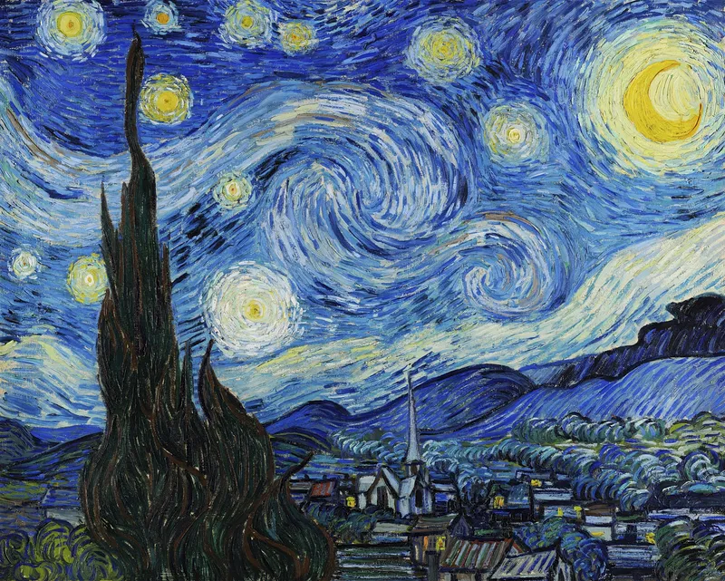
Artists like Claude Monet are recognized for the unique styles of their works, such as the unique colour scheme and brush strokes. These are hard to be imitated by normal people, and even for professional painters, it will not be easy to produce a painting whose style is Monet-esque. However, thanks to the invention of Generative Adversarial Networks (GANs) and their many variations, Data Scientists and Machine Learning Engineers can build and train deep learning models to bring an artist's peculiar style to your photos.

Table of Contents

1. Objectives
2. Setup
   1. Installing Required Libraries
   2. Importing Required Libraries
   3. Defining Helper Functions
3. What is Image Style Transfer in Deep Learning?
4. CycleGANs
   1. A quick recap on vanilla GANs
   2. What's novel about CycleGANs?
5. Data Loading
6. Building the Generator
   1. Defining the Downsampling Block
   2. Defining the Upsampling Block
   3. Assembling the Generator
7. Building the Discriminator
8. Building the CycleGAN Model
9. Defining Loss Functions
10. Model Training
    1. Training the CycleGAN
11. Visualize our Monet-esque photos
    1. Loading the Pre-trained Weights
    2. Visualizing Style Transfer Output

Objectives

In this project I am going to:

• Describe the novelty about CycleGANs
• Define Cycle Consistency Loss
• Describe the complicated architecture of a CycleGAN
• Practice the training deep learning models
• Implement a pre-trained CycleGAN for image style transfer

Setup

For this project, we will be using the following libraries:

• numpy for mathematical operations.
• Pillow for image processing functions.
• tensorflow for machine learning and neural network related functions.
• matplotlib for additional plotting tools.

What is Image Style Transfer in Deep learning?

Image Style Transfer can be viewed as an image-to-image translation, where we "translate" image A into a new image by combining the content of image A with the style of another image B (which could be a famous Monet painting).

CycleGANs

A quick recap on vanilla GANs

GANs are a family of algorithms are use learning by comparison. A vanilla GAN has two parts, a Generator network which we denote by $\boldsymbol G$ and a Discriminator network which we denote by $\boldsymbol D$. $\boldsymbol G$ tries to fool $\boldsymbol D$ through continuously improving its own ability to produce images that are fake but close to the real images. $\boldsymbol D$ is responsible for distinguishing the fake images from the real images and keeps on improving the correctness of its predictions (classifications). Here is a visualization of a vanilla GAN architecture from this publication:

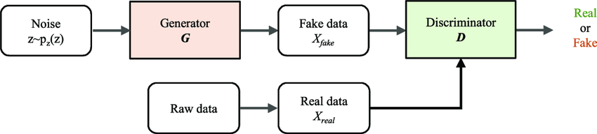
Vanilla GANs use adversarial training to optimize both $\boldsymbol G$ and $\boldsymbol D$ at the same time (well, not quite exactly at the same time but at least both are optimized in one iteration!). In adversatial training, we take into account the losses of both networks when designing the objective function.

What's novel about CycleGANs?

First of all, unlike other GAN models for image-to-image translation, CycleGANs do not require paired training data. For example, if we are interested in translating photographs of winter landscapes to summer landscapes, we do not require each winter landscape to have its corresponding summer view exist in the dataset. This allows the development of image translation models for tasks where paired training datasets are not available.

Besides, CycleGAN uses the additional Cycle Consistency Loss to enforce the forward-backward consistency of the Generators.

What is forward-backward consistency?

As a simple example, if we translate a sentence from English to French, and then translate it back from French to Engligh, we should expect to get back the original english sentence.

Why we need forward-backward consistency?

With one $\boldsymbol G$ that learns a mapping between two domains of images $X$ and $Y$ such that the output $\hat y = \boldsymbol G(x)$ is indistinguishable from $y \in Y$ by $\boldsymbol D$ trained to classify $\hat y$ apart from $y$, we simply can not guarantee that $x$ and $y$ are paired up in a meaningful way. For instance, it probably won't make sense to transfer the style of a Fuji mountain photo in the same way we transfer the style of a cat photo.

Hence, to ensure that the mapping $\boldsymbol G: X \rightarrow Y$ is constrained and meaningful, we introduce a second, inverse mapping $\boldsymbol F: Y \rightarrow X$ to ensure that $F(G(x)) \approx x$ and $G(F(y)) \approx y$, which means an image translation cycle should be able to bring an image back to the original image.

The loss that incurred during the image translation cycle, i.e., the discrepancy between $x$ and $F(G(x))$, $y$ and $G(F(y))$, will be added to the objective function of a CycleGAN as the Cycle Consistency Loss.

Data Loading

The unpaired dataset comes from a Kaggle competition called I'm Something of a Painter Myself. The original dataset contains around 400MB of images, but for this project we will only use 300 Monet paintings and 300 photos for training the CycleGAN. The followinig cell downloads the zipped dataset.

Building the Generator

Defining the Downsampling Block

The CycleGAN Generator model takes an input image and generates an output image. To achieve this, the model architecture begins with a sequence of downsampling convolutional blocks (reduce the 2D dimensions, width and height of an image by the stride) to encode the input image.

To define a downsampling block, we will use the instance normalization method instead of batch normalization as our batch size is very small. InstanceNorm transforms each training sample independently over multiple channels, whereas BatchNorm does that to the whole batch of samples over each channel. The intent is to remove image-specific contrast information from the image, which simplifies the generation and results in better generated images.

Defining the Upsampling Block

Next, the Generator uses a number of Upsampling blocks to generate the output image.

Upsampling does the opposite of downsampling and increases the dimensions of the image. Hence, we use the Conv2DTranspose API from keras to create TransposeConvolution-InstanceNorm-ReLU layers to build the block.

Assembling the Generator

The Generator uses a sequence of downsampling convolutional blocks to encode the input image, a number of residual network (ResNet) convolutional blocks to transform the image, and a number of upsampling convolutional blocks to generate the output image.

The ResNet blocks essentially skip connections to help bypass the vanishing gradient problem through concatenating the output of downsampling layers directly to the output of upsampling layers. You will see that we concatenate them in a symmetrical fashion in the following code cell.

Building the Discriminator

The discriminator model takes a $256 \times 256$ color image and is responsible for classifying it as real or fake. "Fake" as in being produced by the Generator.

This can be implemented directly by borrowing the architecture of a somewhat standard deep convolutional discriminator model. Thus, it can be built by mainly using the Convolution-InstanceNorm-LeakyReLU layers.

Although the InstanceNorm method was designed for generator models, it can also prove effective in discriminator models.

Our Discriminator model will be built using 4 Convolution-InstanceNorm-LeakyReLU layers with 64, 128, 256, and 512 sized 4 filters, respectively. After the last layer, we apply a convolution to produce a 1-dimensional output.

Building the CycleGAN Model

In order to ensure that the mapping between images from two domains is meaningful and desirable, we enforce forward-backward consistency by involving two mappings: $\boldsymbol G: X \rightarrow Y$ and the inverse $\boldsymbol F: Y \rightarrow X$.

This means, our CycleGAN model needs two generators. One for transforming photos to Monet-esque paintings and one for transforming Monet paintings to be more like photos.

Since we have two generators, we would naturally need two discriminators to "discriminate" the work of each of them. This leads to our definition of monet_generator, photo_generator, monet_discriminator, and photo_discriminator in the next cell.

Defining Loss Functions

A perfect discriminator shoud output all 1s for a real image and all 0s for a fake image. Hence, the discriminator_loss compares the discriminator's prediction for a real image to a matrix of 1s and the prediction for a fake image to a matrix of 0s. The differences are quantified using Binary Cross Entropy.

The CycleGAN paper suggests dividing the loss for the discriminator by half during training, in an effort to slow down updates to the discriminator relative to the generator.

Model Training

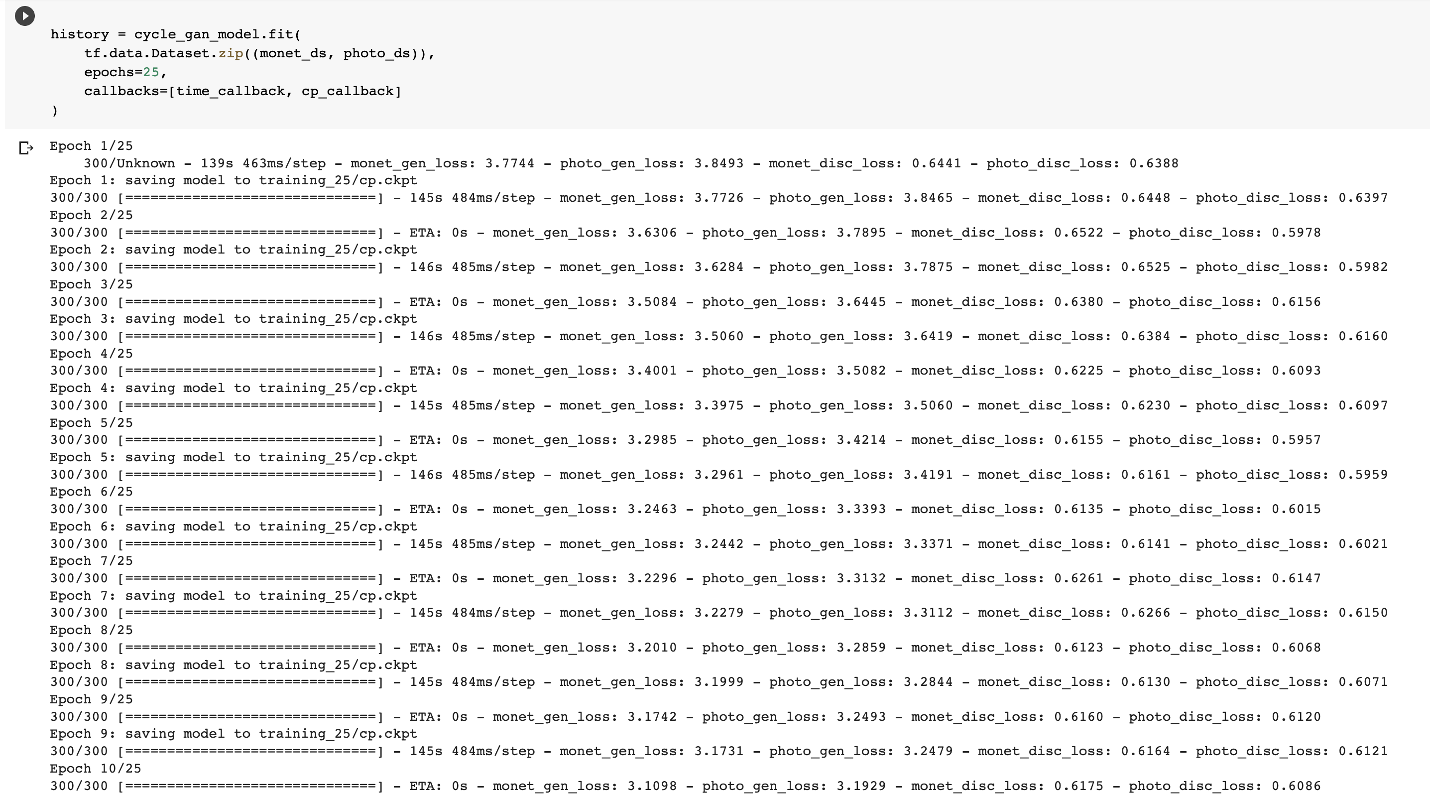
In this section, we will compile and train a CycleGAN. Since our networks have too many parameters (one generator alone has 54M and a discriminator has 2M) and Skills Network Labs currently doesn't have any GPUs available, it will take hours to train a sufficient number of epochs with a CPU such that the model can do a decent job in transfering image styles.

Therefore, we will train the model for one epoch in this lab, which includes 300 iterations.

Visualize our Monet-esque photos

Loading Pre-trained Weights

This is a screenshot of the CycleGAN's training history. Even though only the monet generator is needed for the style transfer task, but we can see that the losses of all 4 networks: monet generator, monet discriminator, photo generator, and photo discriminated, were being optimized.

Visualizing Style Transfer Output

Finally! We will visualize the style transfer output produced by monet_generator_model. We take 5 sample images that are photos of beautiful landscapes in the original dataset and feed them to the model.