(Courtesy: Arpit Verma of Kaggle)
AMC Entertainment Holdings, Inc. (d/b/a AMC Theatres, originally an abbreviation for American Multi-Cinema; often referred to simply as AMC and known in some countries as AMC Cinemas or AMC Multi-Cinemas) is an American movie theater chain headquartered in Leawood, Kansas, and the largest movie theater chain in the world. Founded in 1920, AMC has the largest share of the U.S. theater market ahead of Regal and Cinemark Theatres. After acquiring Odeon Cinemas, UCI Cinemas, and Carmike Cinemas in 2016, it became the largest movie theater chain in the world. It has 2,866 screens in 358 theatres in Europe and 7,967 screens in 620 theatres in the United States.
This dataset provides historical data of AMC Entertainment Holdings, Inc. (AMC). The data is available at a daily level. Currency is USD.
Key:
Date - Actual Date
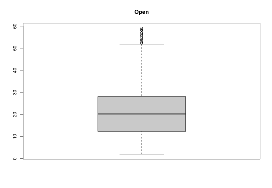
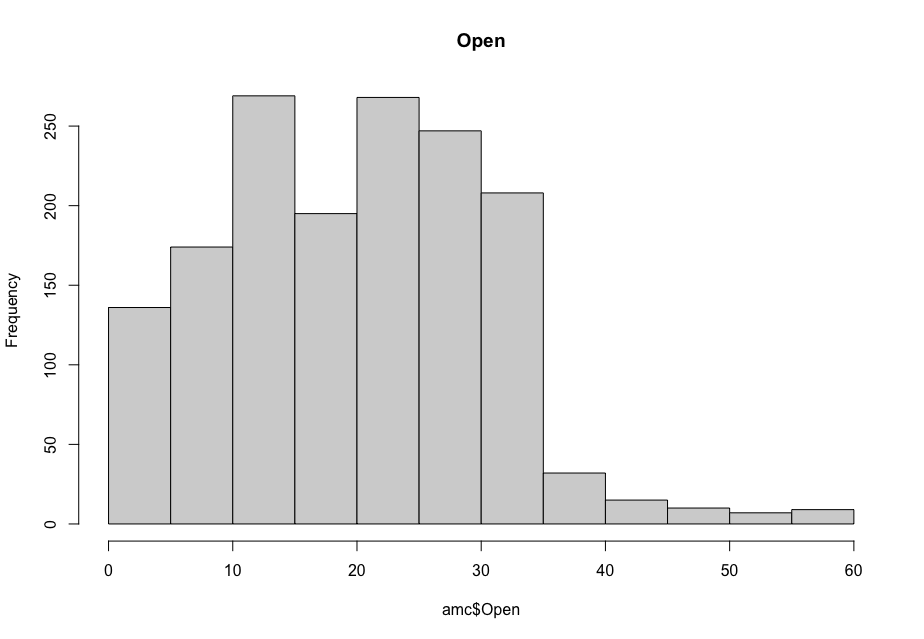
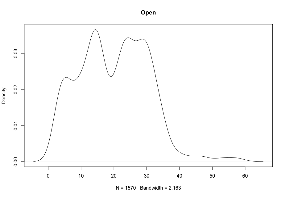
Open - Price from the first transaction of a trading day
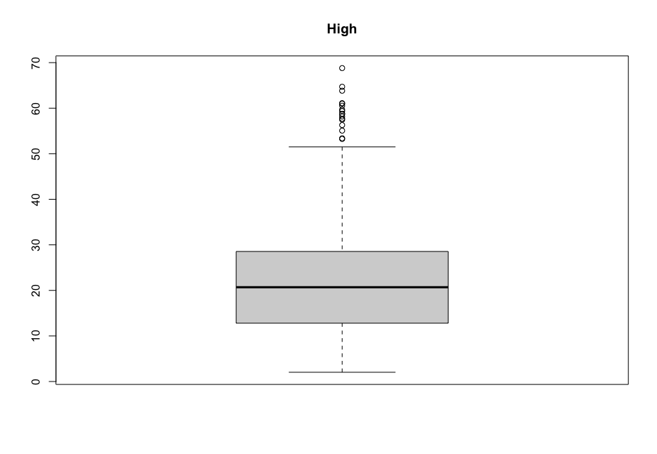
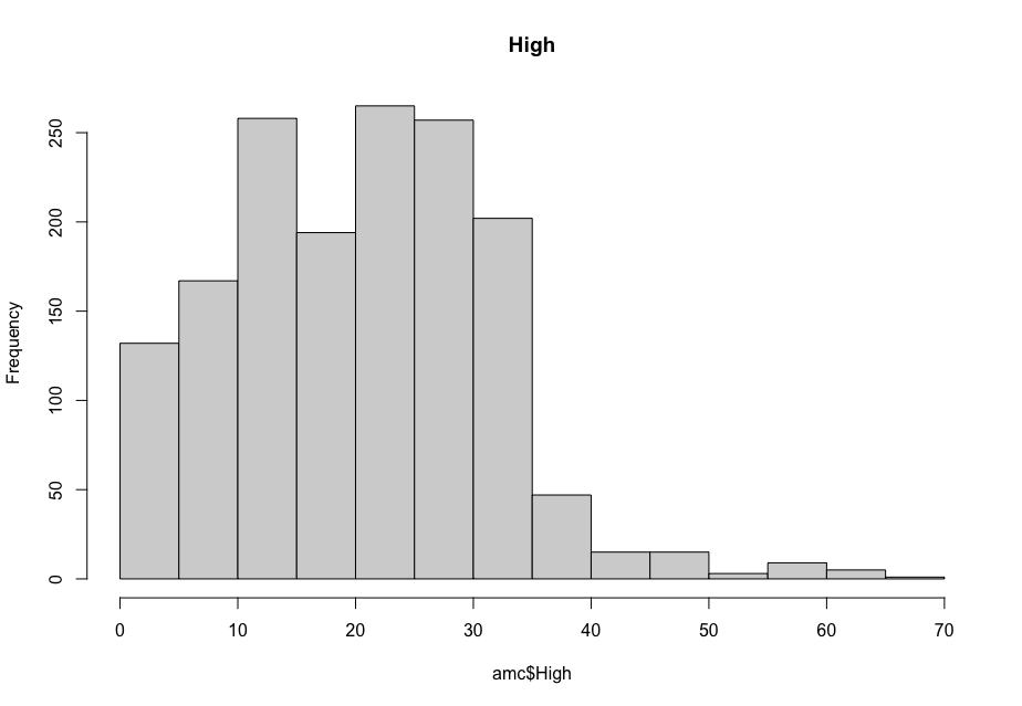
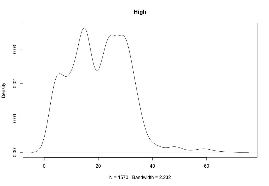
High - Maximum price in a trading day
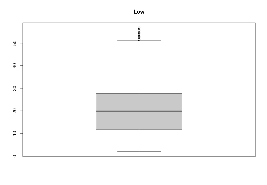
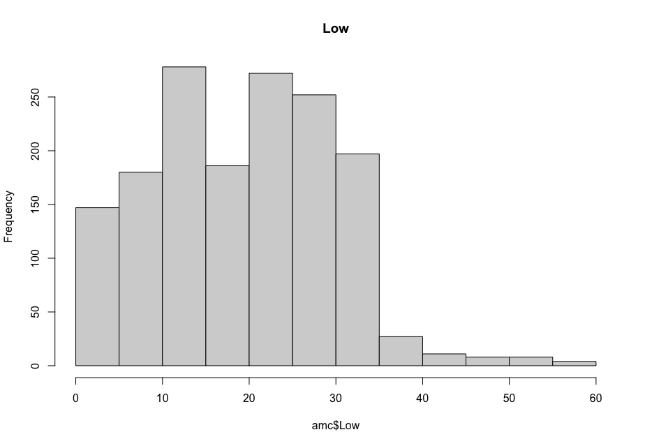
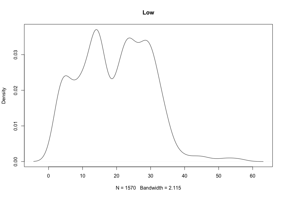
Low - Minimum price in a trading day
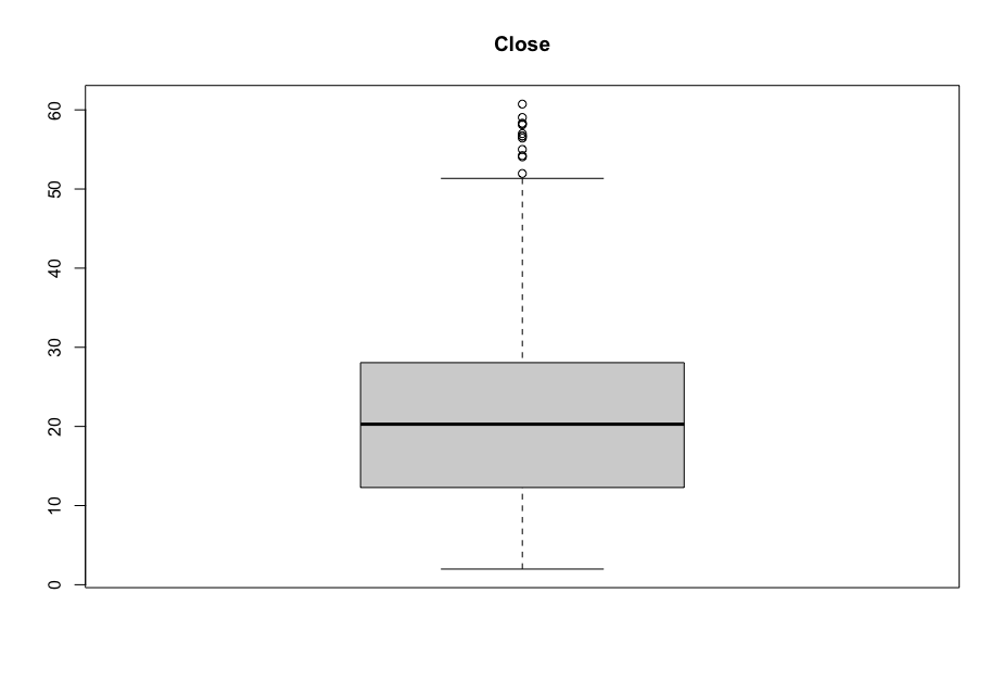
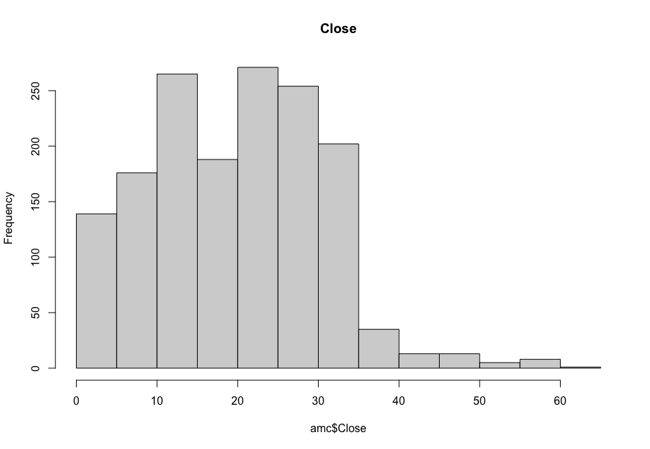
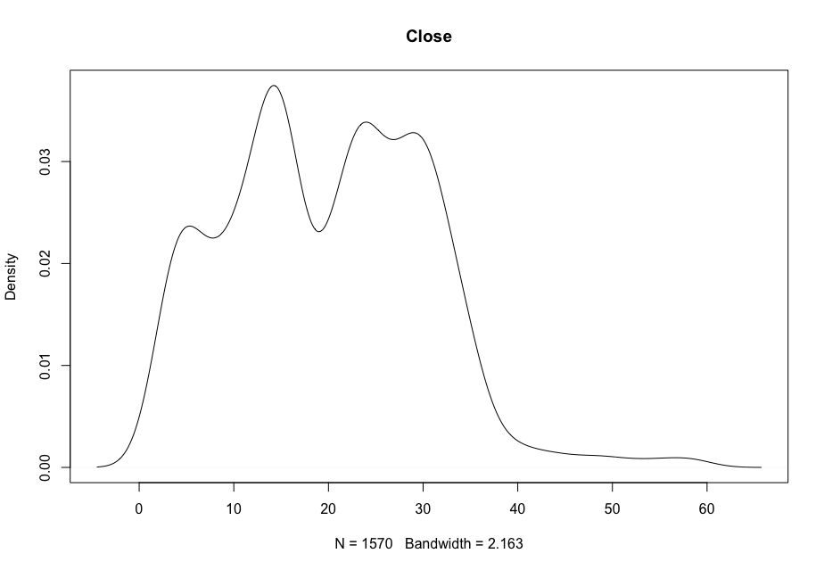
Close - Price from the last transaction of a trading day
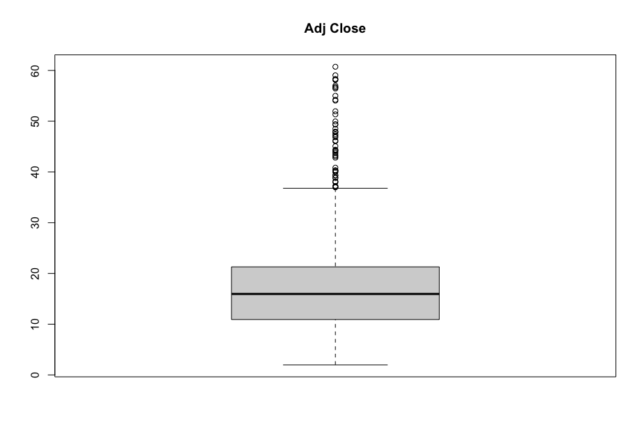
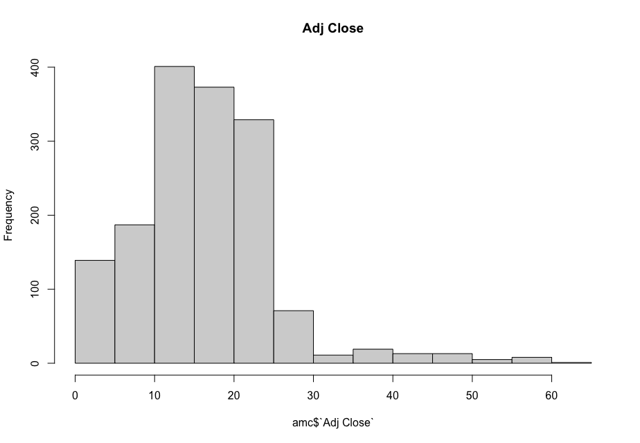
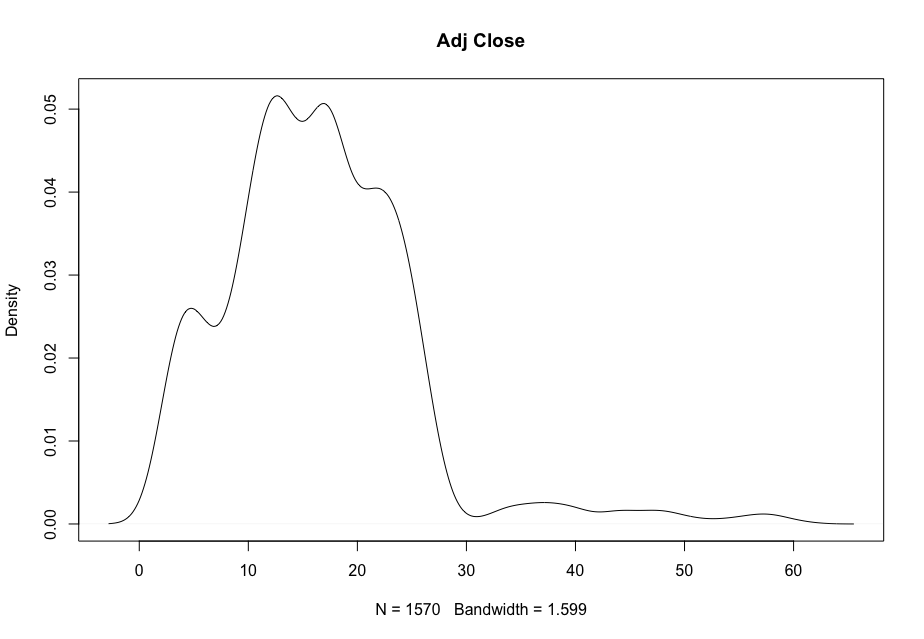
Adj Close - Closing price adjusted to reflect the value after accounting for any corporate actions
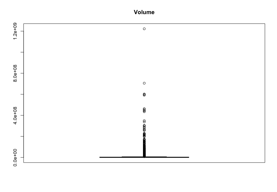
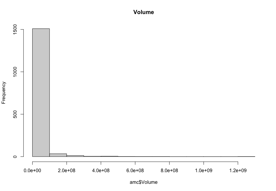
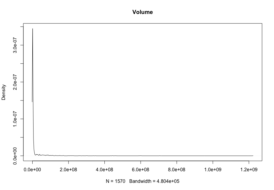
Volume - Number of units traded in a day.
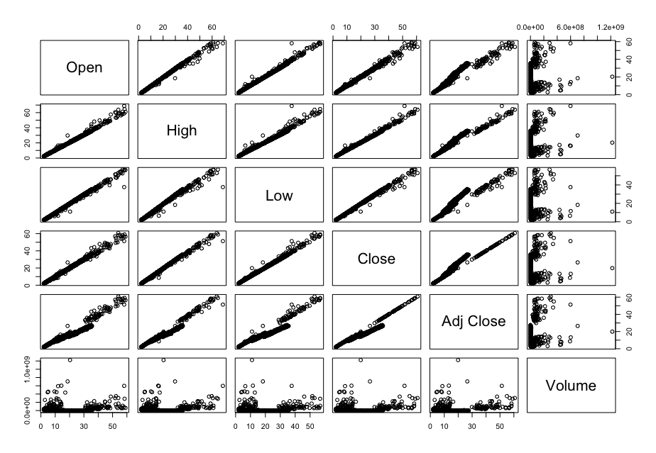
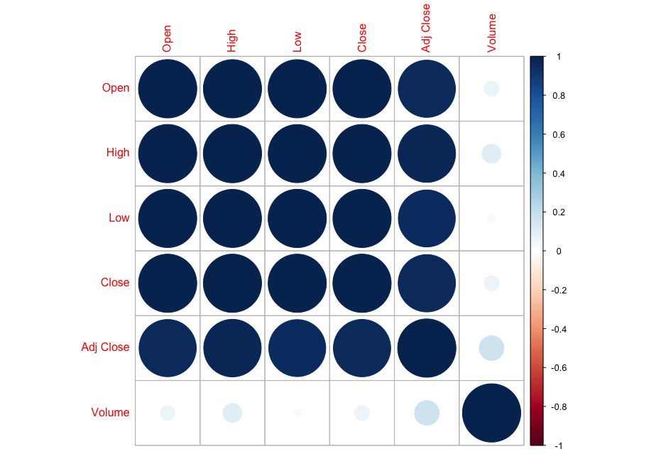
Now, in order to figure out which model works well for this dataset, a validation dataset is generated with 80% of the rows in the original dataset to use for training, with the remaining 20% of the data to be validated. The following graphs monitor the behavior of this training dataset.
In order to figure out which model to use to best predict where the data will trend, we would have to develop a test-harness using 10-fold cross validation with three repeats using various algorithms using various units of measure. The dot-plots showing the performances of each algorithm will be shown below.
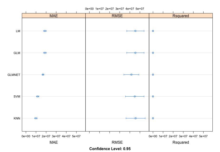
The algorithms in this first outcome are currently centered and scaled with the highly correlated values.
outcome <- resamples(list(LM = fit.lm, GLM = fit.glm, GLMNET = fit.glmnet, SVM = fit.svm, KNN = fit.knn))
summary(outcome)
Call:
summary.resamples(object = outcome)
Models: LM (Linear Model), GLM (Generalized Linear Model), GLMNET (Penalized Linear Model), SVM (Support Vector Machines), KNN (k-Nearest Neighbors)
Number of resamples: 30
MAE
Min. 1st Qu. Median Mean 3rd Qu. Max. NA'sLM 12953051 15748600 18889597 18867085 20288098 28714143 0
GLM 12953051 15748600 18889597 18867085 20288098 28714143 0
GLMNET 12525068 14823381 16795523 16891746 18838886 21194430 0
SVM 5469373 9163424 11043345 11686925 14508471 18779865 0
KNN 3680526 7838716 9201742 9888181 12449735 18141919 0
RMSE
Min. 1st Qu. Median Mean 3rd Qu. Max. NA'sLM 18448670 28932707 39036872 45528957 54000982 90905224 0
GLM 18448670 28932707 39036872 45528957 54000982 90905224 0
GLMNET 15277092 26185167 37147190 41555763 52632754 90660491 0
SVM 7514733 26758981 40627907 44926372 60926524 101696784 0
KNN 11264514 27632479 39947197 45696253 59777525 106387510 0
Rsquared
Min. 1st Qu. Median Mean 3rd Qu. Max. NA'sLM 0.30432783 0.4632728 0.5191817 0.5231661 0.5945303 0.7912763 0
GLM 0.30432783 0.4632728 0.5191817 0.5231661 0.5945303 0.7912763 0
GLMNET 0.31383694 0.4896796 0.5381849 0.5549713 0.6309693 0.8571197 0
SVM 0.32678897 0.4956748 0.5800586 0.5776315 0.7037011 0.8830470 0
KNN 0.03048308 0.3402185 0.5595156 0.4853565 0.6163114 0.8478114 0
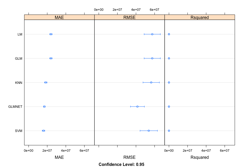
The algorithms in this second outcome are currently centered and scaled without the highly correlated values.
outcome2 <- resamples(list(LM = fit.lm, GLM = fit.glm, GLMNET = fit.glmnet, SVM = fit.svm, KNN = fit.knn))
summary(outcome2)
Call:
summary.resamples(object = outcome2)
Models: LM, GLM, GLMNET, SVM, KNN
Number of resamples: 30
MAE
Min. 1st Qu. Median Mean 3rd Qu. Max. NA'sLM 17120963 21566122 23612492 24000348 26919221 30935049 0
GLM 17120963 21566122 23612492 24000348 26919221 30935049 0
GLMNET 12525068 14823381 16795523 16891746 18838886 21194430 0
SVM 7473668 13559723 15741403 16038858 18803797 23202159 0
KNN 11324251 16083905 17852422 18445773 21068954 24700748 0
RMSE
Min. 1st Qu. Median Mean 3rd Qu. Max. NA'sLM 22152423 40720829 53675120 57491085 72138560 112722853 0
GLM 22152423 40720829 53675120 57491085 72138560 112722853 0
GLMNET 15277092 26185167 37147190 41555763 52632754 90660491 0
SVM 11644364 35641578 48940324 53708943 69864280 111750830 0
KNN 22902736 38815155 48411236 56359413 72153949 111490350 0
Rsquared
Min. 1st Qu. Median Mean 3rd Qu. Max. NA'sLM 1.483748e-05 0.0009268357 0.006890912 0.01918216 0.03102276 0.08289168 0
GLM 1.483748e-05 0.0009268357 0.006890912 0.01918216 0.03102276 0.08289168 0
GLMNET 3.138369e-01 0.4896796108 0.538184948 0.55497133 0.63096929 0.85711975 0
SVM 6.511007e-03 0.0458225992 0.142131962 0.20097528 0.30306220 0.71290539 0
KNN 7.462957e-03 0.0339076231 0.121907488 0.14276862 0.21591304 0.51108661 0
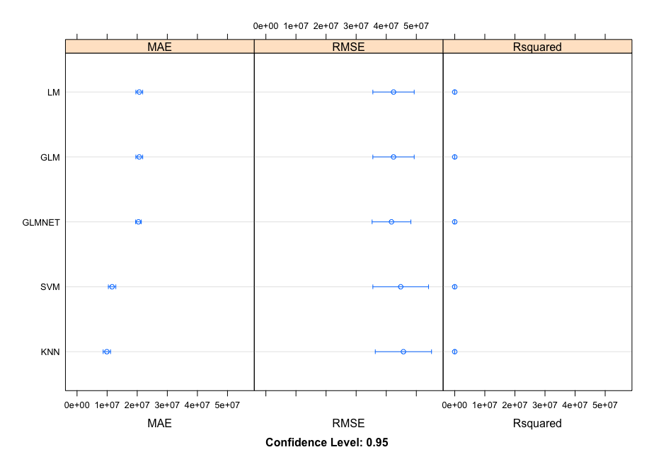
The algorithms in this third outcome are currently centered, scaled, and transformed using the Box-Cox method with the highly correlated values.
outcome3 <- resamples(list(LM = fit.lm, GLM = fit.glm, GLMNET = fit.glmnet, SVM = fit.svm, KNN = fit.knn))
summary(outcome3)
Call:
summary.resamples(object = outcome3)
Models: LM, GLM, GLMNET, SVM, KNN
Number of resamples: 30
MAE
Min. 1st Qu. Median Mean 3rd Qu. Max. NA'sLM 14317954 19166740 20684487 20684035 22974526 26701879 0
GLM 14317954 19166740 20684487 20684035 22974526 26701879 0
GLMNET 15919979 18634403 20616042 20416441 22130482 24761106 0
SVM 5680386 8945198 10876737 11650119 14548465 18924878 0
KNN 4032008 7916614 9216504 9910743 12324078 17621998 0
RMSE
Min. 1st Qu. Median Mean 3rd Qu. Max. NA'sLM 20952996 29348149 36896169 42420653 49173955 94586011 0
GLM 20952996 29348149 36896169 42420653 49173955 94586011 0
GLMNET 20668753 29614356 36502576 41740995 48523019 87240671 0
SVM 7826026 26266721 39953805 44807230 60338621 102646673 0
KNN 13423914 28075877 39029866 45705324 59636949 104705672 0
Rsquared
Min. 1st Qu. Median Mean 3rd Qu. Max. NA'sLM 0.20995793 0.4161312 0.5313362 0.5180253 0.6168191 0.8587488 0
GLM 0.20995793 0.4161312 0.5313362 0.5180253 0.6168191 0.8587488 0
GLMNET 0.21172570 0.4511238 0.5180361 0.5098385 0.5880617 0.7885906 0
SVM 0.29198507 0.4809362 0.5704306 0.5699200 0.7150422 0.8766482 0
KNN 0.02963859 0.3563041 0.5478481 0.4798609 0.6387612 0.8239043 0
Three additional ensemble outcomes are added to improve the analysis of analyzing the data, all of which are transformed via the Box-Cox method.
ensemble <- resamples(list(RF = fit.rf, GBM = fit.gbm, CUBIST = fit.cubist))
summary(ensemble)
Call:
summary.resamples(object = ensemble)
Models: RF (Random Forest), GBM (Gradient Booster Method), CUBIST
Number of resamples: 30
MAE
Min. 1st Qu. Median Mean 3rd Qu. Max. NA'sRF 5665450 7472449 8695215 9341970 11044333 14681649 0
GBM 10711818 13155020 14458774 14632866 16536161 18984534 0
CUBIST 3757394 5768194 7417536 7440709 8955991 12277018 0
RMSE
Min. 1st Qu. Median Mean 3rd Qu. Max. NA'sRF 16168780 22975529 32974827 38079897 48155583 70467545 0
GBM 20919656 27326500 36363300 42106731 52561442 88884199 0
CUBIST 10527833 17260591 24987716 31072433 41017138 67678798 0
Rsquared
Min. 1st Qu. Median Mean 3rd Qu. Max. NA'sRF 0.1021230 0.5789694 0.6794716 0.6267992 0.7462763 0.8697522 0
GBM 0.1110092 0.4715421 0.5421579 0.5268957 0.6505939 0.7527193 0
CUBIST 0.1621931 0.6962783 0.7533742 0.7322539 0.8724464 0.9536887 0
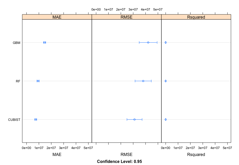
The aim for picking the most efficient model is to find the model with the lowest root mean square error (RMSE). There's also a mean absolute error (MAE) & an r-squared error. However, our main concern is the RMSE. Overall, given the data that is shown above, it is proven that the Cubist model would be the best model to run the data.
#Cubist Wins#
#Look deeper into winning model#
print(fit.cubist)
Cubist
1570 samples
5 predictors . Pre-processing: Box-Cox transformation (5)
Resampling: Cross-Validated (10 fold, repeated 3 times)
Summary of sample sizes: 1413, 1414, 1413, 1414, 1412, 1412, ...
Resampling results across tuning parameters:
committees neighbors RMSE Rsquared MAE
1 0 45728962 0.4990559 10291250
1 5 44921116 0.5135953 10035744
1 9 45045970 0.5123765 10115521
10 0 35877489 0.6351564 8310675
10 5 35542554 0.6366793 8500939
10 9 35559963 0.6389609 8574697
20 0 35253899 0.6521506 8158116
20 5 34942691 0.6501143 8382772
20 9 34929826 0.6531267 8448448
RMSE was used to select the optimal model using the smallest value.
The final values used for the model were committees = 20 and neighbors = 9.
#Train the Final Model#
library(Cubist)
set.seed(7)
x <- amc[,1:5]
y <- amc[,6]
preprocessParams <- preProcess(x)
tX <- sample(1:nrow(amc), floor(.8*nrow(amc)))
p <- c("Open", "High", "Low", "Close", "Adj Close")
tXp <- amc[tX, p]
tXr <- amc$Volume[tX]
fM <- cubist(x = tXp, y = tXr, commitees = 20, neighbors = 9)
fM
summary(fM)
predictions <- predict(fM, tXp)
#Compute the RMSE & R^2#
rmse <- sqrt(mean((predictions - tXr)^2))
r2 <- cor(predictions, tXr)^2
print(rmse) #17255498# - RMSE Value
print(r2) #0.903859# - R2 Value
In closing, this model above will most likely work for this type of regressive dataset. But, please also take note that those values fluctuate every day. Therefore, you still want to make sure to compare each and every algorithms to find the best possible model to generate a prediction of when the next price and volume will be.
Copyright (c) 2021 Robert (Christian) Paul & Arpit Verma
Permission is hereby granted, free of charge, to any person obtaining a copy of this software and associated documentation files (the "Software"), to deal in the Software without restriction, including without limitation the rights to use, copy, modify, merge, publish, distribute, sublicense, and/or sell copies of the Software, and to permit persons to whom the Software is furnished to do so, subject to the following conditions:
The above copyright notice and this permission notice shall be included in all copies or substantial portions of the Software.
THE SOFTWARE IS PROVIDED "AS IS", WITHOUT WARRANTY OF ANY KIND, EXPRESS OR IMPLIED, INCLUDING BUT NOT LIMITED TO THE WARRANTIES OF MERCHANTABILITY, FITNESS FOR A PARTICULAR PURPOSE AND NONINFRINGEMENT. IN NO EVENT SHALL THE AUTHORS OR COPYRIGHT HOLDERS BE LIABLE FOR ANY CLAIM, DAMAGES OR OTHER LIABILITY, WHETHER IN AN ACTION OF CONTRACT, TORT OR OTHERWISE, ARISING FROM, OUT OF OR IN CONNECTION WITH THE SOFTWARE OR THE USE OR OTHER DEALINGS IN THE SOFTWARE.