A data structure is a particular way of organizing data in a computer so that it can be used effectively. The idea is to reduce the space and time complexities of different tasks.
Below is an overview of some popular linear data structures.
- Array
- Linked List
- Stack
- Queue
- Binary Tree
- Binary Search Tree
- Graph
Array is a data structure used to store homogeneous elements at contiguous locations. Size of an array must be provided before storing data.
Let size of array be n.
Accessing Time : O(1) [This is possible because elements are stored at contiguous locations]
Search Time : O(n) for Sequential Search; O(log n) for Binary Search [If Array is sorted]
Insertion Time : O(n) [The worst case occurs when insertion happens at the Beginning of an array and requires shifting all of the elements]
Deletion Time : O(n) [The worst case occurs when deletion happens at the Beginning of an array and requires shifting all of the elements]
A linked list is a linear data structure (like arrays) where each element is a separate object. Each element (that is node) of a list is comprising of two items – the data and a reference to the next node.
-
Singly Linked List : In this type of linked list, every node stores address or reference of next node in list and the last node has next address or reference as NULL. For example 1->2->3->4->NULL
-
Doubly Linked List : In this type of Linked list, there are two references associated with each node, One of the reference points to the next node and one to the previous node. Advantage of this data structure is that we can traverse in both the directions and for deletion we don’t need to have explicit access to previous node. Eg. NULL<-1<->2<->3->NULL
-
Circular Linked List : Circular linked list is a linked list where all nodes are connected to form a circle. There is no NULL at the end. A circular linked list can be a singly circular linked list or doubly circular linked list. Advantage of this data structure is that any node can be made as starting node. This is useful in implementation of circular queue in linked list. Eg. 1->2->3->1 [The next pointer of last node is pointing to the first]
Accessing Time : O(n)
Search Time : O(n)
Insertion Time : O(1) [If we are at the position where we have to insert an element]
Deletion Time : O(1) [If we know address of node previous the node to be deleted]
A stack or LIFO (last in, first out) is an abstract data type that serves as a collection of elements, with two principal operations: push, which adds an element to the collection, and pop, which removes the last element that was added. In stack both the operations of push and pop takes place at the same end that is top of the stack. It can be implemented by using both array and linked list.
Insertion Time : O(1)
Deletion Time : O(1)
Access Time : O(n) [Worst Case]
Note: Insertion and Deletion are allowed on one end.
A queue or FIFO (first in, first out) is an abstract data type that serves as a collection of elements, with two principal operations: enqueue, the process of adding an element to the collection.(The element is added from the rear side) and dequeue, the process of removing the first element that was added. (The element is removed from the front side). It can be implemented by using both array and linked list.
Insertion Time : O(1)
Deletion Time : O(1)
Access Time : O(n) [Worst Case]
Note: Circular Queue:- The advantage of this data structure is that it reduces wastage of space in case of array implementation, As the insertion of the (n+1)’th element is done at the 0’th index if it is empty.
Unlike Arrays, Linked Lists, Stack and queues, which are linear data structures, trees are hierarchical data structures. A binary tree is a tree data structure in which each node has at most two children, which are referred to as the left child and the right child. It is implemented mainly using Links.
A tree is represented by a pointer to the topmost node in tree. If the tree is empty, then value of root is NULL. A Binary Tree node contains following parts.
- Data
- Pointer to left child
- Pointer to right child
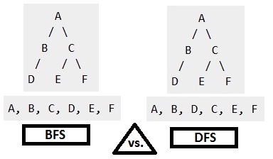
A Binary Tree can be traversed in two ways:
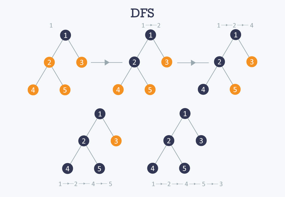
- Depth First Traversal: Inorder (Left-Root-Right), Preorder (Root-Left-Right) and Postorder (Left-Right-Root)
- Breadth First Traversal: Level Order Traversal
The maximum number of nodes at level ‘l’ = 2l-1.
Maximum number of nodes = 2h – 1. [Here h is height of a tree. Height is considered as is maximum number of nodes on root to leaf path]
Minimum possible height = ceil(Log2(n+1))
In Binary tree, number of leaf nodes is always one more than nodes with two children.
Time Complexity of Tree Traversal = O(n)
In Binary Search Tree is a Binary Tree with following additional properties:
- The left subtree of a node contains only nodes with keys less than the node’s key.
- The right subtree of a node contains only nodes with keys greater than the node’s key.
- The left and right subtree each must also be a binary isExists tree.
Search : O(h)
Insertion : O(h)
Deletion : O(h)
Extra Space : O(n) for pointers
Note:
h: Height of BST
n: Number of nodes in BST
BST provide moderate access/isExists (quicker than Linked List and slower than arrays).
BST provide moderate insertion/deletion (quicker than Arrays and slower than Linked Lists).
Graph is a data structure that consists of following two components:
-
A finite set of vertices also called as nodes.
-
A finite set of ordered pair of the form (u, v) called as edge. The pair is ordered because (u, v) is not same as (v, u) in case of directed graph(di-graph). The pair of form (u, v) indicates that there is an edge from vertex u to vertex v. The edges may contain weight/value/cost.
V -> Number of Vertices.
E -> Number of Edges.
Graph can be classified on the basis of many things, below are the two most common classifications :
- Direction
Undirected Graph : The graph in which all the edges are bidirectional.
Directed Graph : The graph in which all the edges are unidirectional.
- Weight
Weighted Graph : The Graph in which weight is associated with the edges.
Unweighted Graph : The Graph in which their is no weight associated to the edges.
Graph can be represented in many ways, below are the two most common representations :
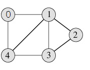
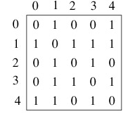
- 1: Adjacency Matrix
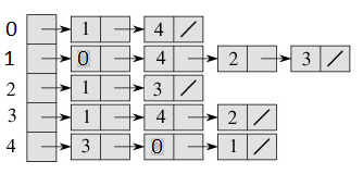
- 2: Adjacency List
Time Complexities in case of Adjacency Matrix :
Traversal : By BFS or DFS) O(V^2)
Space : O(V^2)
Time Complexities in case of Adjacency List :
Traversal : (By BFS or DFS) O(ElogV)
Space : O(V+E)
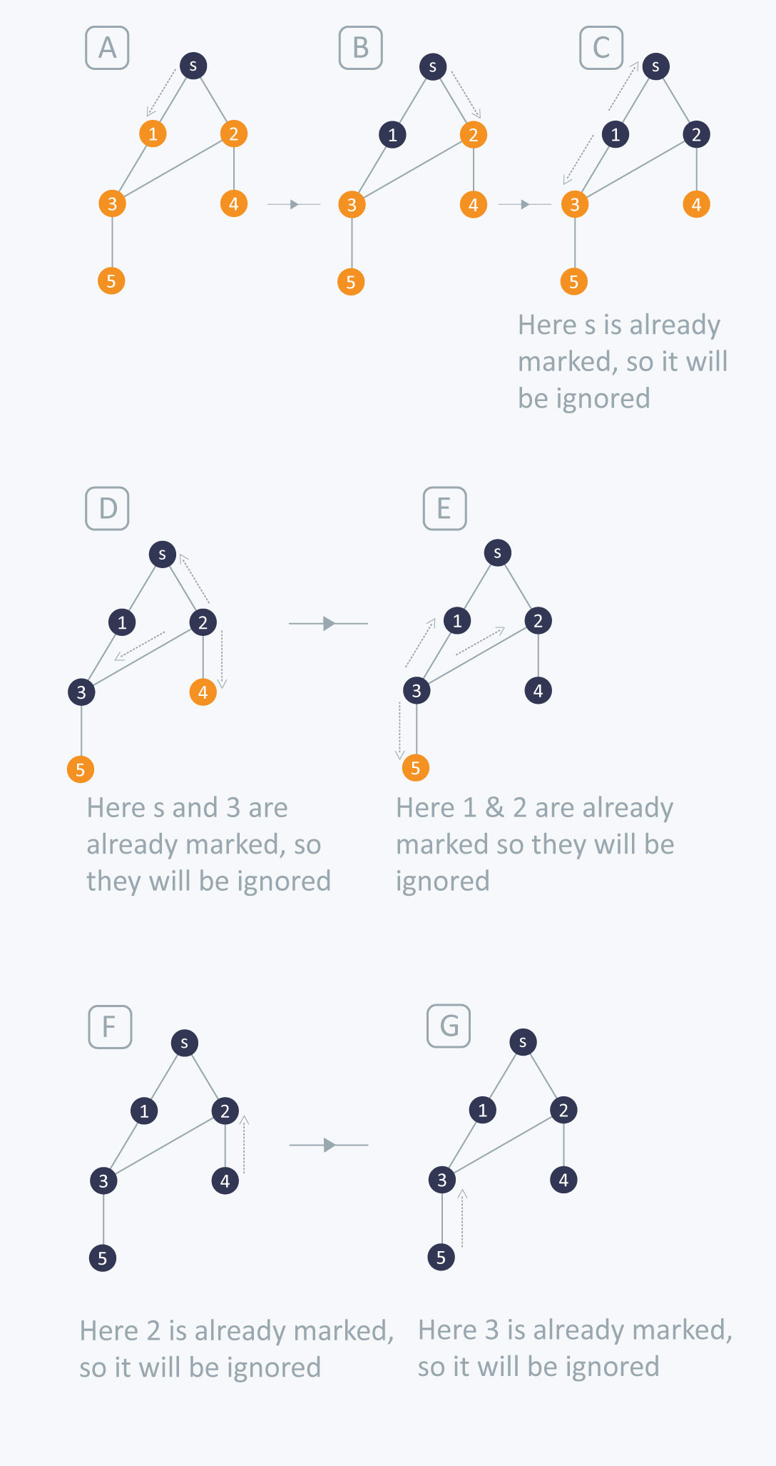
The DFS algorithm is a recursive algorithm that uses the idea of backtracking. It involves exhaustive searches of all the nodes by going ahead, if possible, else by backtracking.
Here, the word backtrack means that when you are moving forward and there are no more nodes along the current path, you move backwards on the same path to find nodes to traverse. All the nodes will be visited on the current path till all the unvisited nodes have been traversed after which the next path will be selected.
This recursive nature of DFS can be implemented using stacks. The basic idea is as follows:
- Pick a starting node and push all its adjacent nodes into a stack.
- Pop a node from stack to select the next node to visit and push all its adjacent nodes into a stack.
- Repeat this process until the stack is empty. However, ensure that the nodes that are visited are marked. This will prevent you from visiting the same node more than once. If you do not mark the nodes that are visited and you visit the same node more than once, you may end up in an infinite loop.
The following image shows how BFS works.
    DFS-iterative (G, s):                                   //Where G is graph and s is source vertex
      let S be stack
      S.push( s )            //Inserting s in stack
      mark s as visited.
      while ( S is not empty):
          //Pop a vertex from stack to visit next
          v  =  S.top( )
         S.pop( )
         //Push all the neighbours of v in stack that are not visited
        for all neighbours w of v in Graph G:
            if w is not visited :
                     S.push( w )
                    mark w as visited


    DFS-recursive(G, s):
        mark s as visited
        for all neighbours w of s in Graph G:
            if w is not visited:
                DFS-recursive(G, w)
O(V + E), when implemented using an adjacency list.
BFS is a traversing algorithm where you should start traversing from a selected node (source or starting node) and traverse the graph layer-wise thus exploring the neighbour nodes (nodes which are directly connected to source node). You must then move towards the next-level neighbour nodes.
As the name BFS suggests, you are required to traverse the graph breadth-wise as follows:
- First move horizontally and visit all the nodes of the current layer
- Move to the next layer
Consider the following diagram:
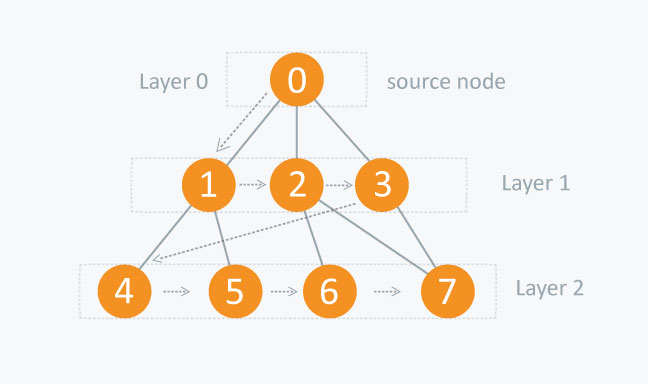
The distance between the nodes in layer 1 is comparitively lesser than the distance between the nodes in layer 2. Therefore, in BFS, you must traverse all the nodes in layer 1 before you move to the nodes in layer 2.
A graph can contain cycles, which may bring you to the same node again while traversing the graph. To avoid processing of same node again, use a boolean array which marks the node after it is processed. While visiting the nodes in the layer of a graph, store them in a manner such that you can traverse the corresponding child nodes in a similar order.
In the earlier diagram, start traversing from 0 and visit its child nodes 1, 2, and 3. Store them in the order in which they are visited. This will allow you to visit the child nodes of 1 first (i.e. 4 and 5), then of 2 (i.e. 6 and 7), and then of 3 (i.e. 7) etc.
To make this process easy, use a queue to store the node and mark it as 'visited' until all its neighbours (vertices that are directly connected to it) are marked. The queue follows the First In First Out (FIFO) queuing method, and therefore, the neigbors of the node will be visited in the order in which they were inserted in the node i.e. the node that was inserted first will be visited first, and so on.
The following image shows how BFS works.
BFS (G, s)                   //Where G is the graph and s is the source node
      let Q be queue.
      Q.enqueue( s ) //Inserting s in queue until all its neighbour vertices are marked.

      mark s as visited.
      while ( Q is not empty)
           //Removing that vertex from queue,whose neighbour will be visited now
           v  =  Q.dequeue( )

          //processing all the neighbours of v
          for all neighbours w of v in Graph G
               if w is not visited
                        Q.enqueue( w )             //Stores w in Q to further visit its neighbour
                        mark w as visited.
The time complexity of BFS is O(V + E), where V is the number of nodes and E is the number of edges.
| BFS | DFS |
|---|---|
| BFS visit nodes level by level in Graph. | DFS visit nodes of graph depth wise. It visits nodes until reach a leaf or a node which doesn’t have non-visited nodes. |
| A node is fully explored before any other can begin. | Exploration of a node is suspended as soon as another unexplored is found. |
| Uses Queue data structure to store Un-explored nodes. | Uses Stack data structure to store Un-explored nodes. |
| BFS is slower and require more memory. | DFS is faster and require less memory. |
| Some Applications: | Some Applications: |
| - Finding all connected components in a graph. | - Topological Sorting |
| - Finding the shortest path between two nodes. | - Finding connected components |
| - Finding all nodes within one connected component. | - Solving puzzles such as maze |
| - Testing a graph for bipartiteness. | - Finding strongly connected components |
| - Finding articulation points (cut vertices) of the graph. |
Example
Considering A as starting vertex.