Repository navigation
1 sEEG CCEP ds004696
Single-pulse electrical stimulation through pairs of neighbouring stereo-EEG contacts, and the responses it evokes at every other contact, analysed through the iEEGLAB menus: from the recording to the response of each site-contact pair, the connectivity matrix, time-frequency power and a bipolar montage. The participant is sub-02 of OpenNeuro ds004696 (Ojeda Valencia et al., 2023).
Each step gives the menu, what you should get (Expect), the window or figure that opens, and the same step from the command line. The screenshots are from the tutorial extract. Install iEEGLAB first (Installation).
Two versions of the same recording; the steps give the numbers of both where they differ.
-
Tutorial extract: nothing to download, a few minutes for all the steps.
tutorial/seegin the iEEGLAB folder holds an extract at the native sampling rate with its BIDS sidecar files: 17 contacts, 3 stimulation sites, 34 pulses. - Full recording: sub-02 from OpenNeuro, with the AWS command line (no account needed) or from ds004696. Keep the folder structure. Reading it needs the MEF3 plugin (File > Manage EEGLAB extensions).
aws s3 sync --no-sign-request s3://openneuro.org/ds004696 ds004696 --exclude "*" --include "sub-02/*" --include "derivatives/freesurfer/sub-02/*" --include "dataset_description.json" --include "participants.tsv"
The files the steps use, in the BIDS folder structure (ses-ieeg01 is the session, ieeg the data type):
ds004696/
  dataset_description.json, participants.tsv
  sub-02/ses-ieeg01/ieeg/
    sub-02_ses-ieeg01_task-ccep_run-01_ieeg.mefd       the recording (a folder; step 1)
    sub-02_ses-ieeg01_task-ccep_run-01_channels.tsv    contact types and bad contacts (step 2)
    sub-02_ses-ieeg01_task-ccep_run-01_events.tsv      the stimulations and their sites (step 2)
    sub-02_ses-ieeg01_electrodes.tsv                   contact coordinates (step 2)
    sub-02_ses-ieeg01_coordsystem.json                 the space of the coordinates (step 3)
  derivatives/freesurfer/sub-02/
    pial.L.surf.gii, pial.R.surf.gii                   the participant's brain surfaces (step 3)
The tutorial extract has the same sidecar files and pial surfaces, with the .set dataset in place of the .mefd
recording, all in one folder, tutorial/seeg.
Note. The full recording needs about 20 GB of memory, and CARLA takes 6 to 7 minutes. For a quicker run, read only a few stimulation sites at step 1; the numbers then differ a little, also for the sites you keep, as CARLA and the permutations draw from one random stream. The times on this page come from a Windows laptop with 8 cores; a recent Mac (Apple M5 Pro) was as fast or up to 3.5 times faster.
Tutorial extract: File > Load existing dataset: in the iEEGLAB folder,
tutorial/seeg/sub-02_ses-ieeg01_task-ccep_run-01_ieeg.set.
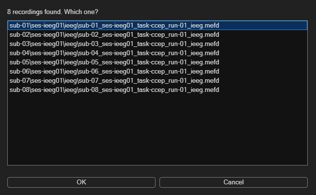
Full recording: iEEGLAB > Import raw recording: select the ds004696 folder, then sub-02's recording. Keep the
defaults.
Expect.
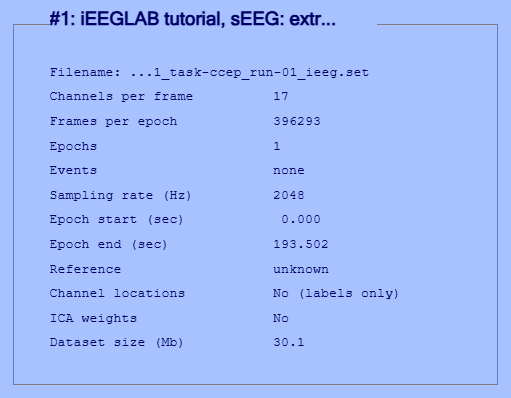
- Tutorial extract: 17 channels at 2048 Hz, 3.2 minutes.
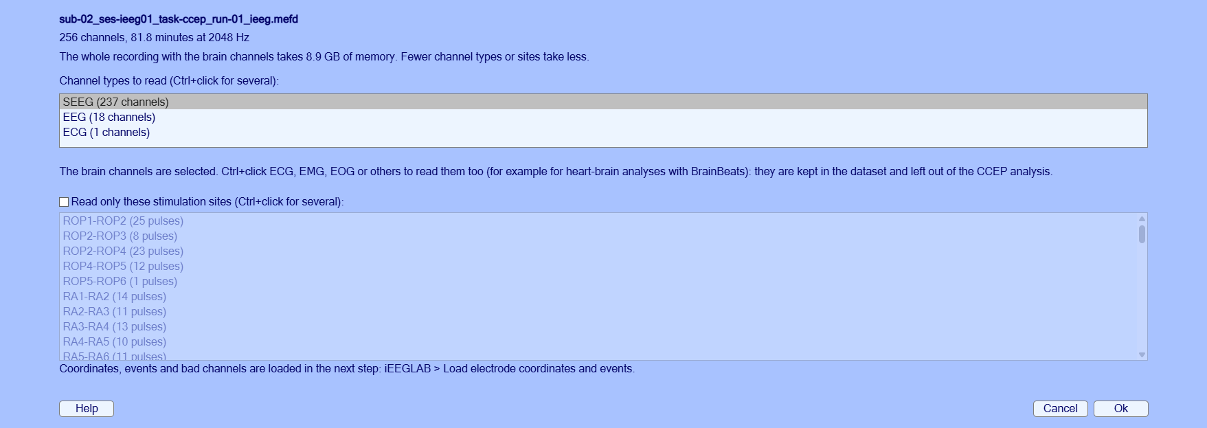
- Full recording: About 1.5 minutes, with the progress in the command window and a progress bar: 237 channels at 2048 Hz.
Full recording, the two import windows:
% Tutorial extract
tut = fullfile(fileparts(which('eegplugin_ieeglab')), 'tutorial', 'seeg');
EEG = pop_loadset('filename', 'sub-02_ses-ieeg01_task-ccep_run-01_ieeg.set', 'filepath', tut);
% Full recording
rec = fullfile('ds004696', 'sub-02', 'ses-ieeg01', 'ieeg', 'sub-02_ses-ieeg01_task-ccep_run-01_ieeg.mefd');
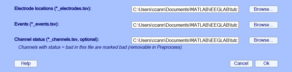
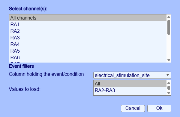
EEG = ieeglab_import(rec); % or ieeglab_import(rec, 'sites', {'RA2-RA3', 'RA3-RA4'})iEEGLAB > Load electrode coordinates and events: Ok in both windows. The sidecar files next to the dataset are
found automatically; the event type is the stimulation site (for example RA3-RA4), and the contacts marked bad in
channels.tsv are marked here and removed during preprocessing.
Note. After this step and most of the next ones (and after the import of the full recording), EEGLAB asks what to do with the result (window Dataset info -- pop_newset()). By default, Ok keeps the result as a new dataset, under the name shown, and the previous one in memory (Datasets menu). Tick Overwrite it in memory to replace the previous one instead: with the full recording, each copy takes 9 to 16 GB (the 20 GB of the note above are for one copy at a time). Tick Save it as file to also write the result to disk.
Expect.
- Tutorial extract: 14 of 17 contacts with coordinates, 3 bad (RA15, RB14, RB15, from
channels.tsv), 34 stimulations at 3 sites. A warning says that the same three have no position in the electrodes file.- Full recording: 211 contacts with coordinates, 39 bad (from
channels.tsv), 695 stimulations.
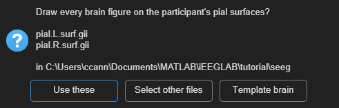
EEG = ieeglab_load(EEG, struct('event_field', 'electrical_stimulation_site'));iEEGLAB > Choose brain surfaces: Use these (sub-02's pial surfaces), then iEEGLAB > Visualize electrodes.
Chosen once, the surfaces are used by every brain figure. Without a choice, figures are drawn on the brain that matches
the space of the coordinates in coordsystem.json: the participant's pial surfaces for participant coordinates (ACPC
here), fsaverage's for fsaverage or MNI coordinates.
The window names the files it found: pial.L.surf.gii and pial.R.surf.gii, in tutorial/seeg for the tutorial
extract and in ds004696/derivatives/freesurfer/sub-02 for the full recording. If it offers Select pial files
instead of Use these, the surfaces were not downloaded or not kept in that folder: select these two files.
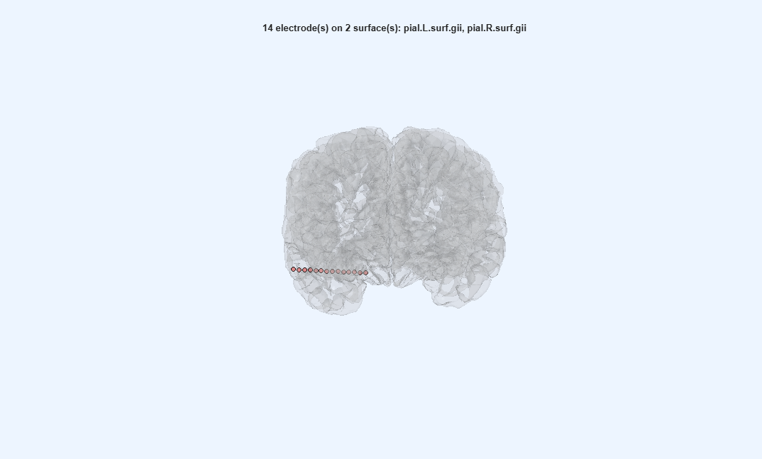
Expect. The contacts inside the brain, seen from the front and slightly above; drag to rotate. The tutorial extract shows one lead (RA), in the right hemisphere.
EEG = pop_ieeglab_surfaces(EEG, 'surf_files', ieeglab_brain_surfaces(EEG));
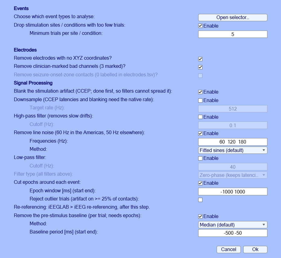
EEG = ieeglab_vis_elec(EEG);iEEGLAB > Preprocess iEEG data: tick Reject outlier trials, keep the rest: artifact blanking, line noise at 60, 120 and 180 Hz removed by fitted sines, no filter (a notch or a high-pass spreads each response around the pulse), epochs -1 to 1 s, baseline -500 to -50 ms; sites with fewer than 5 pulses, bad contacts and contacts without coordinates removed.
Expect.
- Tutorial extract: A few seconds: 14 contacts, 32 epochs. The command window names RA14 as not flat before the pulse: it is kept, as the clinicians marked it good.
- Full recording: About a minute: 198 contacts, 627 epochs.
Note. Line noise: the fitted sines were compared with a notch filter, ZapLine (de Cheveigné, 2020) and ZapLine-plus (Klug & Kloosterman, 2022), on synthetic stimulation data with a known clean signal and on both datasets. They left the least error 5 to 50 ms after the pulse (0.1 µV, against 0.5 µV for the notch and 19 to 20 µV for ZapLine), and are the default. Details in the help of
ieeglab_line_noise.
EEG = ieeglab_preprocess(EEG, struct('apply_blank', true, 'apply_notch', true, 'notch', [60 120 180], ...
    'apply_epoch', true, 'epoch_window', [-1000 1000], 'reject_trials', true, ...
    'remove_rare_cond', true, 'min_trials', 5, 'remove_no_coords', true, ...
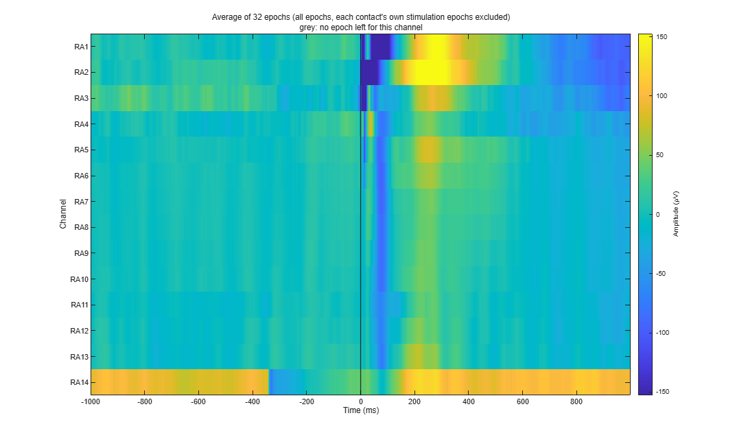
'remove_bad_channels', true, 'apply_baseline', true, 'baseline_period', [-500 -50]));iEEGLAB > Plot average of epochs, every channel (heatmap). It works at any step once the data are epoched.
Expect. One row per contact, the average of all epochs in colour: flat before 0 ms, responses after it. In the tutorial extract, RA14 is the row that is not flat before 0 ms.
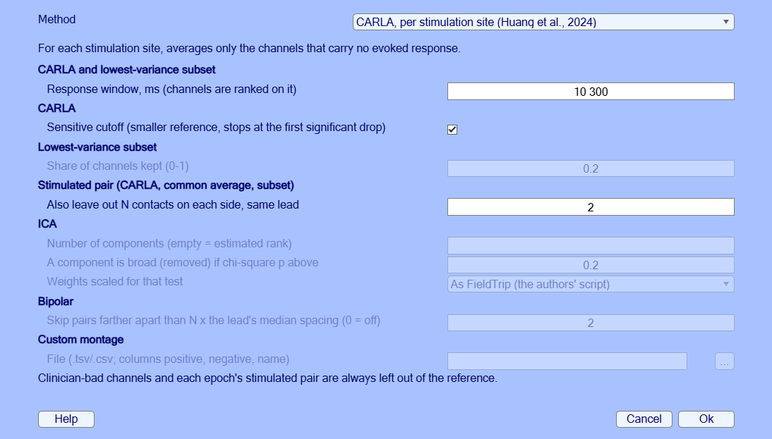
ieeglab_plot_heatmap(EEG);iEEGLAB > iEEG re-referencing: CARLA, defaults. CARLA chooses, for each stimulation site, the channels whose common average carries no evoked response (Huang et al., 2024). The defaults are its authors' settings for real data: sensitive cutoff; the stimulated pair, 2 contacts on each side of it and bad contacts left out.
Expect.
- Tutorial extract: A few seconds for the 3 sites.
- Full recording: 6 to 7 minutes for the 57 sites.
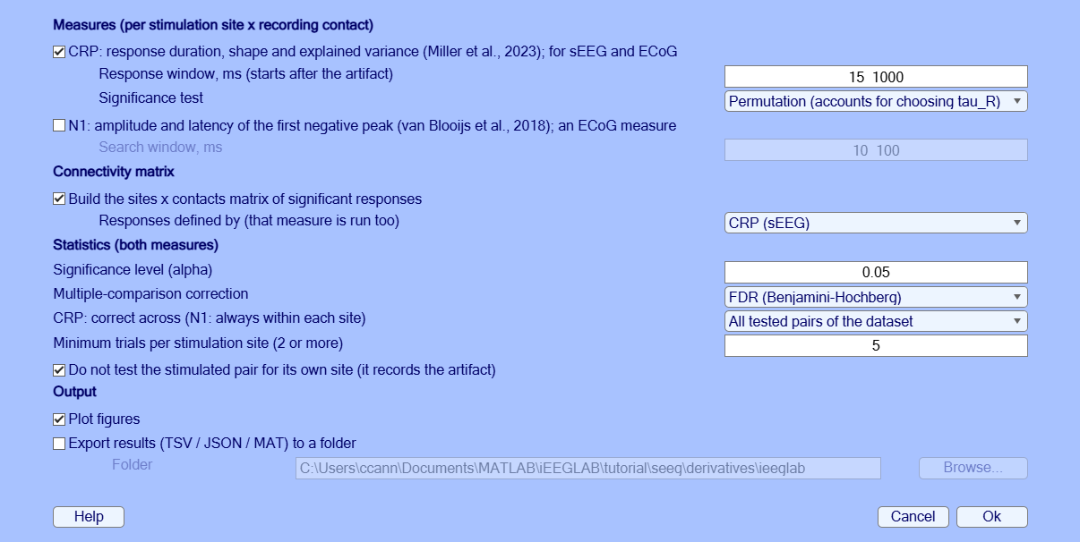
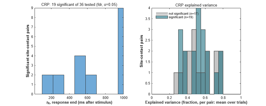
EEG = pop_ieeglab_reref(EEG, 'method', 'carla');iEEGLAB > CCEP analysis: defaults (CRP on the samples after 15 ms up to 1 s, as in the authors' code; matrix from CRP). On sEEG the response of each site-contact pair is described by the Canonical Response Parameterization (CRP; Miller et al., 2023): its duration, shape and explained variance, with a permutation test. The connectivity matrix collects the significant responses.
Expect. The results repeat exactly from run to run on the same data (fixed random seed).
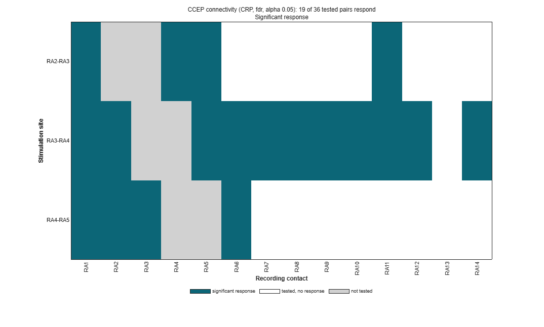
- Tutorial extract: A few seconds: 19 of 36 site-contact pairs respond (the stimulation sites are next to each other on one lead, so most contacts respond).
- Full recording: Under a minute: 3937 of 10780 site-contact pairs respond. A warning says that 392 more cannot reach significance, at sites with too few trials, and count as not tested. Against the published CRP of this participant: the same decision for 83% of the 484 published pairs tested here. With the paper's own settings, iEEGLAB reaches the paper's decision on all 484; Re-referencing compared gives what each setting changes.
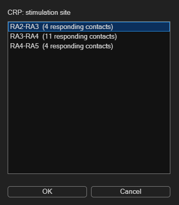
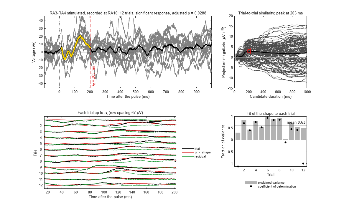
EEG = ieeglab_stats_subject(EEG, struct('run_n1', false, 'run_crp', true, 'run_matrix', true, 'matrix_source', 'crp'));Tutorial extract: iEEGLAB > Plot CRP of one site and contact: RA3-RA4, then RA10.
Full recording: iEEGLAB > Plot CRP of one site and contact: RX4-RX5, then RF2.
The figure shows one pair as in Miller et al. (2023): the trials and their average up to the response duration, the trial-to-trial similarity, each trial with the fitted shape, and the fit per trial.
Expect.
- Tutorial extract: Response duration 203 ms; the shape explains on average 63% of each trial's variance.
- Full recording: Response duration 232 ms (published: 234 ms); the shape explains on average 98% of each trial's variance.
% Tutorial extract
ieeglab_plot_crp(EEG, 'RA3-RA4', 'RA10');
% Full recording
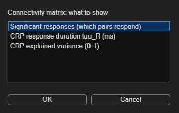
ieeglab_plot_crp(EEG, 'RX4-RX5', 'RF2');iEEGLAB > Plot connectivity matrix: Significant responses, then CRP explained variance.
Expect. Each row is a stimulated pair, each column a recording contact; a cell shows whether stimulating that pair evoked a response at that contact. Teal: a significant response; white: tested, no response; grey: not tested (the stimulated contacts themselves, bad contacts, sites with too few trials). Read a row to see where a site's stimulation reaches, a column to see which sites reach a contact. The second view colours the responding pairs by CRP explained variance, how much of each trial the response shape explains (0 to 1).
- Tutorial extract: 3 sites by 14 contacts.
- Full recording: 57 sites by 198 contacts.
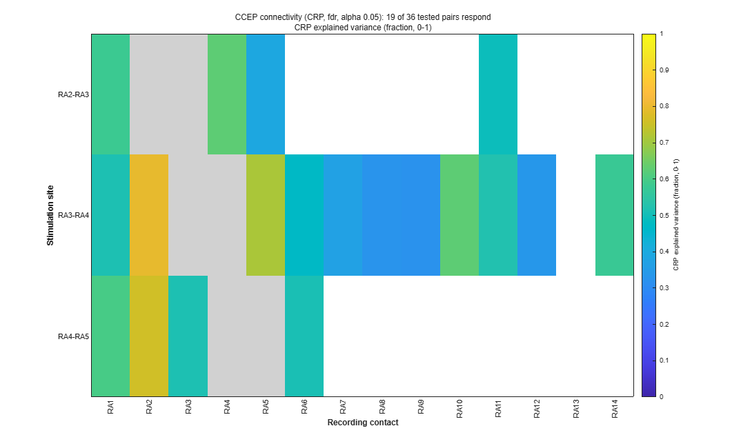
pop_ieeglab_ccep_matrix(EEG, 'response');
pop_ieeglab_ccep_matrix(EEG, 'explained_var');iEEGLAB > Plot electrode values on brain: In-degree.
Expect. Each contact coloured by the number of sites that evoke a response there.
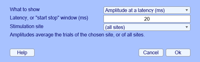
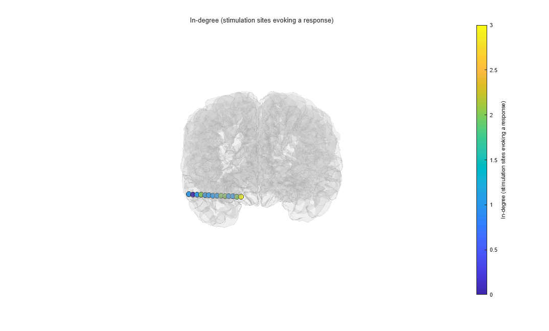
pop_ieeglab_topoplot(EEG, 'in_degree');iEEGLAB > Export results: choose a folder.
Expect. TSV tables (BIDS derivatives style), a JSON record of every option used, and a MAT file.
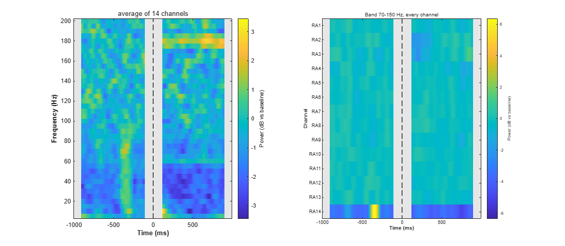
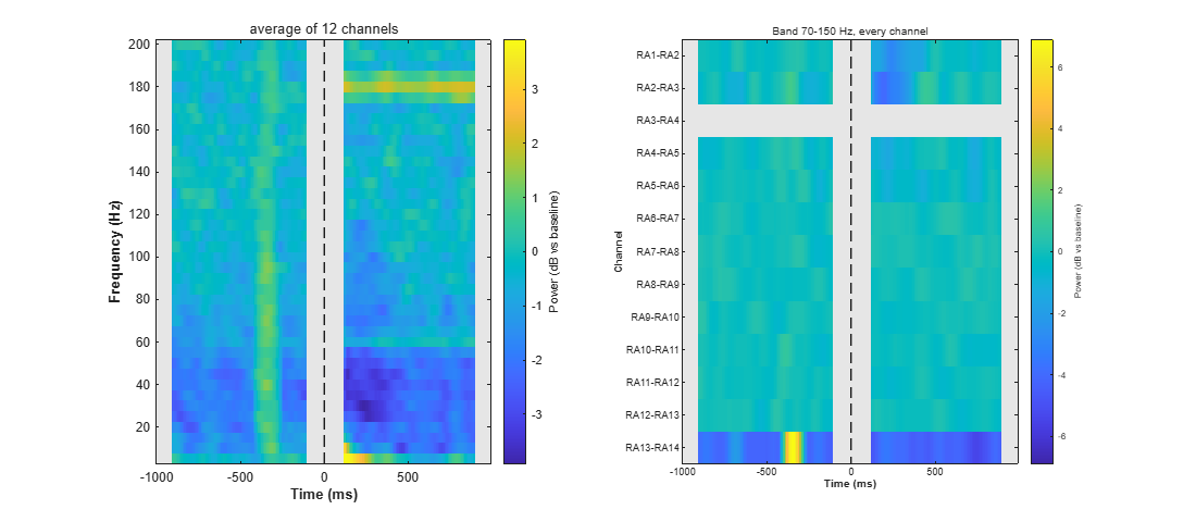
ieeglab_export(EEG, 'results_seeg');iEEGLAB > Frequency analysis: Time-frequency power and band power, keep the defaults (5 to 200 Hz, Hann windows of 0.2 s, dB against the baseline, high-frequency activity 70-150 Hz). It only draws figures: the dataset is not changed. Then, optionally, the same again with Test each contact's band power in this window against its baseline ticked.
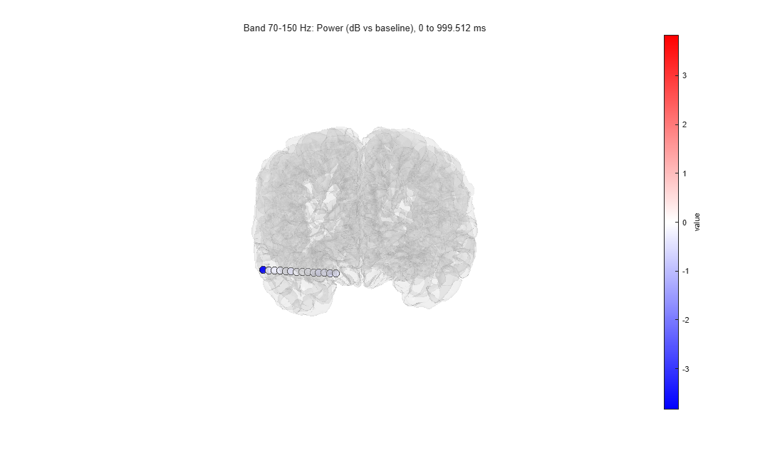
Expect. Two figures. The first shows the power of the average of the contacts over time and frequency, and the 70-150 Hz power of every contact over time; the second, each contact's 70-150 Hz power from 0 to 1000 ms on the brain. The times from -100 to 110 ms are grey: a window that contains the pulse shows power at every frequency. Each contact's own stimulation epochs are left out of its average.
- Tutorial extract: Over 0 to 1000 ms, the 70-150 Hz power of every contact but RA14 is 0.1 dB (RA7) to 0.5 dB (RA4) below its baseline (median -0.3 dB). RA14 is 3.8 dB below: a burst of power about 350 ms before the pulse (the bright patch in its row) raises its baseline, and it also makes the stripe at that time and most of the blue below 60 Hz after the pulse in the average. The grey band covers the first 110 ms, where the responses to a single pulse are largest. With Window 0.1 s the map starts at 70 ms.
- Full recording: Over 0 to 1000 ms, every contact's 70-150 Hz power is between 0.3 dB below (RF13) and 0.4 dB above (RZ1) its baseline (median 0.0 dB), except RA14 (1.7 dB below) and LX12 (1.4 dB below).
Expect, with the test. Each contact's 70-150 Hz change from 0 to 1000 ms is tested against its baseline over the epochs (sign-flip permutation, false discovery rate across contacts). The command window gives the count, the second panel stars the contacts that differ (when it names each contact: 60 or fewer), and the brain shows only them, or every contact's tested change when none differs.
- Tutorial extract: No contact differs (smallest corrected p 0.20). The test averages each epoch's change in dB: for RA14 it is -0.2 dB, where the average power, which the burst in its baseline dominates, gives -3.8 dB. RA3, with 9 epochs, cannot reach significance after the correction and is marked not testable.
- Full recording: About 2 minutes; the single-epoch band power takes about 1.7 GB of memory. No contact differs (smallest corrected p 0.06).
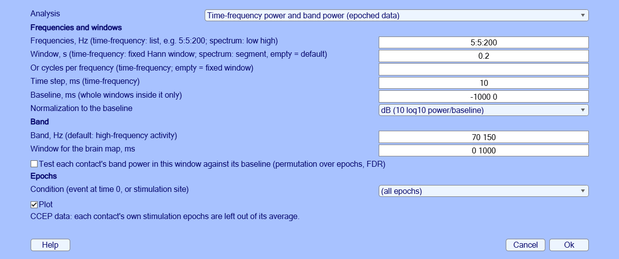
EEG = pop_ieeglab_spectral(EEG, 'type', 'timefreq');
EEG = pop_ieeglab_spectral(EEG, 'type', 'timefreq', 'stats', true); % with the testiEEGLAB > Frequency analysis: Power spectrum of each contact, keep the defaults.
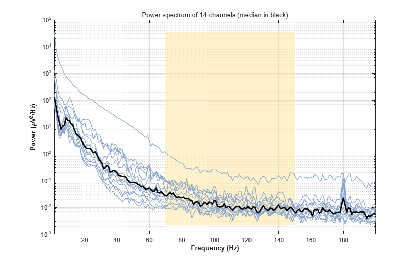
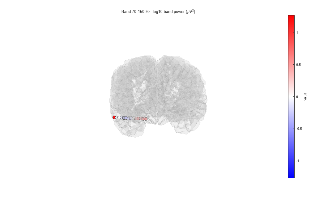
Expect. One curve per contact on a log scale, their median in black, falling steeply with frequency, and the 70-150 Hz power on the brain. On stimulation epochs the spectrum uses only the part before the pulse: the 1 s window is shortened to 0.95 s, one segment per epoch.
- Tutorial extract: No peak at 60 or 120 Hz in the median: the line noise was removed. One is left at 180 Hz (about 3.5 times the neighbouring frequencies in the median); the largest is on RA3 (40 times), next to the stimulated pairs.
- Full recording: No peak at the line frequency or its harmonics in the median: the line noise was removed. The largest peaks left are on LB3, at 60 Hz (20 times the neighbouring frequencies) and 180 Hz (12 times).
EEG = pop_ieeglab_spectral(EEG, 'type', 'spectrum');iEEGLAB > iEEG re-referencing: choose Bipolar in Method, keep the default (on depth leads every consecutive pair is formed; the distance check applies to grids and strips).
Expect. Each contact minus the next one on its lead, at the midpoint of the two. The CCEP results are removed: they describe the old channels. A bipolar difference cancels any reference common to its two contacts, so the same channels come from the CARLA data as from the preprocessed ones.
- Tutorial extract: The 14 contacts become 13 channels, RA1-RA2 to RA13-RA14.
- Full recording: The 198 contacts become 178 channels, from the 197 that have a neighbour (ROP4 has none: ROP3 and ROP5 are bad). Most leads hold groups of contacts 3.3 to 4.2 mm apart with gaps of 7 to 14 mm between groups; 21 channels span such a gap (e.g. LB5-LB6, RB5-RB6).
EEG = pop_ieeglab_reref(EEG, 'method', 'bipolar');iEEGLAB > Frequency analysis again: Time-frequency power and band power, on the bipolar channels.
Expect. As in step 12, one row per bipolar channel.
- Tutorial extract: RA3-RA4 has no value: RA3 or RA4 is stimulated in every epoch (sites RA2-RA3, RA3-RA4 and RA4-RA5). RA13-RA14 is 4.3 dB below its baseline (RA14's burst again), RA1-RA2 1.0 dB and RA2-RA3 0.8 dB below; the others are between -0.5 and +0.1 dB.
- Full recording: Every channel stays within 0.3 dB of its baseline (highest: RZ1-RZ2), except RA13-RA14 (2.2 dB below) and LX11-LX12 (0.7 dB below).
EEG = pop_ieeglab_spectral(EEG, 'type', 'timefreq');If a result differs from Expect or from the picture, a step fails, or a window is unclear, please open an issue with the message and the MATLAB command window, and the MATLAB and EEGLAB versions and operating system.
- de Cheveigné, A. (2020). ZapLine: A simple and effective method to remove power line artifacts. NeuroImage, 207, 116356.
- Huang, H., Ojeda Valencia, G., Gregg, N. M., Osman, G. M., Montoya, M. N., Worrell, G. A., Miller, K. J., & Hermes, D. (2024). CARLA: Adjusted common average referencing for cortico-cortical evoked potential data. Journal of Neuroscience Methods, 407, 110153.
- Klug, M., & Kloosterman, N. A. (2022). Zapline-plus: A Zapline extension for automatic and adaptive removal of frequency-specific noise artifacts in M/EEG. Human Brain Mapping, 43(9), 2743-2758.
- Miller, K. J., Müller, K.-R., Ojeda Valencia, G., Huang, H., Gregg, N. M., Worrell, G. A., & Hermes, D. (2023). Canonical response parameterization: Quantifying the structure of responses to single-pulse intracranial electrical brain stimulation. PLOS Computational Biology, 19(5), e1011105.
- Ojeda Valencia, G., Gregg, N. M., Huang, H., Lundstrom, B. N., Brinkmann, B. H., Pal Attia, T., Van Gompel, J. J., Bernstein, M. A., In, M.-H., Huston, J., III, Worrell, G. A., Miller, K. J., & Hermes, D. (2023). Signatures of electrical stimulation driven network interactions in the human limbic system. Journal of Neuroscience, 43(39), 6697-6711.