Repository navigation
5 CARLA ds004977
CARLA (common average referencing by least anticorrelation; Huang et al., 2024) chooses, for each stimulation site, the channels whose common average carries no evoked response. This page applies it through the iEEGLAB menus to the recording of the paper's Figure 5, with the authors' settings: sub-1 of OpenNeuro ds004977, stereo-EEG at 4800 Hz, stimulation site RMO8-RMO9. The authors' code puts 154 of 206 channels in the common average there; iEEGLAB chooses the same 154. The page then compares CARLA with the common average of all 206 good channels.
Each step gives the menu, what you should get (Expect), and the same step from the command line. Install iEEGLAB first (Installation).
Run 2 of sub-1, from OpenNeuro, with the AWS command line (no account needed) or from ds004977: 304 MB. Keep the folder structure. Reading it needs the MEF3 plugin (File > Manage EEGLAB extensions).
aws s3 sync --no-sign-request s3://openneuro.org/ds004977 ds004977 --exclude "*" --include "sub-1/ses-ieeg01/ieeg/*run-02*" --include "sub-1/ses-ieeg01/ieeg/*_electrodes.tsv" --include "sub-1/ses-ieeg01/ieeg/*_coordsystem.json" --include "dataset_description.json" --include "participants.tsv" --include "task-ccep_events.json"
Note. The public dataset holds only the samples behind the paper's Figures 1 to 6; the other samples are 0 (see its README). In run 2, only the 12 pulses at RMO8-RMO9 have data: the other 9 sites import without an error but are flat, so this page keeps RMO8-RMO9 only. The dataset has no pial surfaces (its FreeSurfer folder holds the T1 and labels), so the page has no brain figure: iEEGLAB > Visualize electrodes would draw the contacts on a template brain, which does not line up with these coordinates (ACPC, the participant's own space).
Steps 1 to 4 take about a minute on a Windows laptop with 8 cores. The recording takes under 3 GB of memory.
iEEGLAB > Import raw recording: select the ds004977 folder, then sub-1's run 2
(sub-1_ses-ieeg01_task-ccep_run-02_ieeg.mefd). Keep the defaults: the whole recording, brain channels only.
Expect. About 25 seconds, with the progress in the command window and a progress bar: 255 stereo-EEG channels at 4800 Hz, 9 minutes.
Note. Read only these stimulation sites (RMO8-RMO9) in the import options reads 44 seconds instead of 9 minutes. The high-pass filter of step 3 then works on that stretch, which changes the covariance of a few channels a little: CARLA still chooses 154 channels, but RP17 instead of RP14, its 154th and 155th channels. Read the whole recording to reproduce the paper exactly.
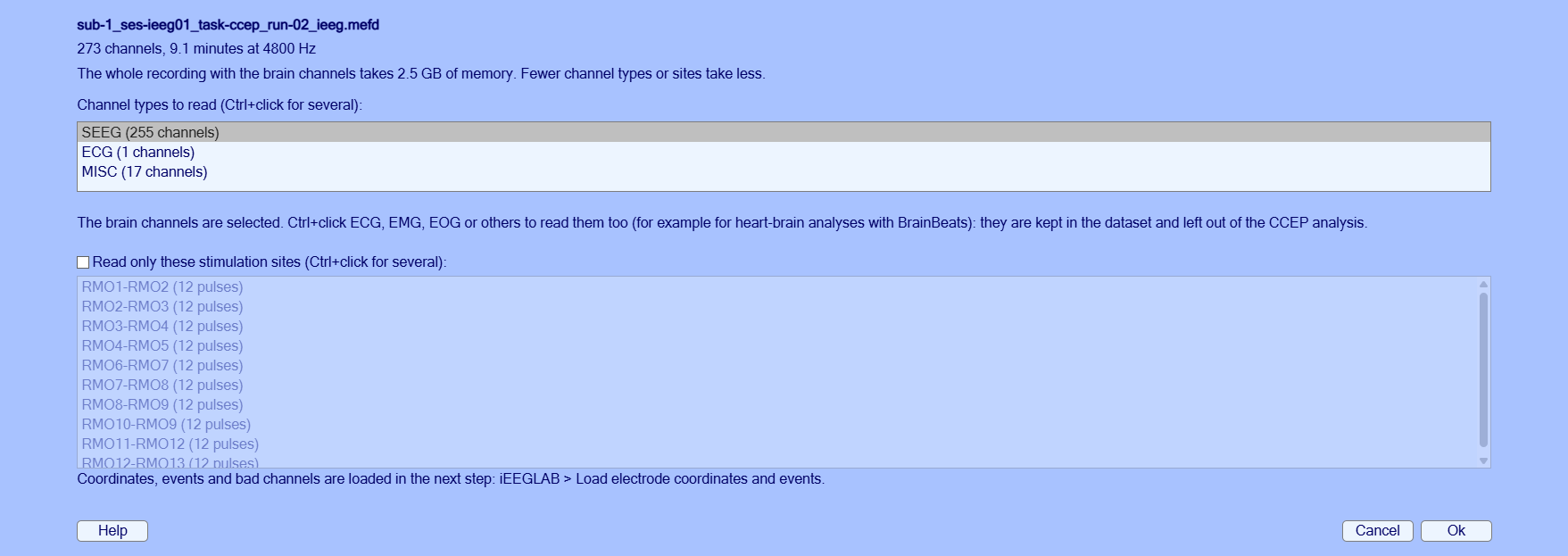
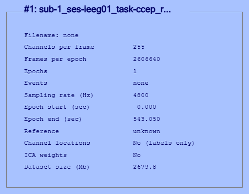
rec = fullfile('ds004977', 'sub-1', 'ses-ieeg01', 'ieeg', 'sub-1_ses-ieeg01_task-ccep_run-02_ieeg.mefd');
EEG = ieeglab_import(rec);iEEGLAB > Load electrode coordinates and events: Ok in both windows. The sidecar files next to the recording are
found automatically; the event type is the stimulation site, and the contacts marked bad in channels.tsv are marked
here and removed during preprocessing.
Expect. 228 of 255 contacts with coordinates, 43 bad (from
channels.tsv), 120 stimulations at 10 sites. A warning names the 27 contacts with no position inelectrodes.tsv: 25 of them are bad, the other two are RP18 and ROC14.
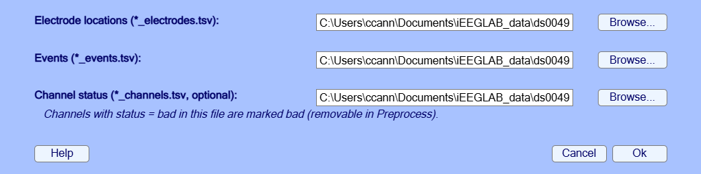
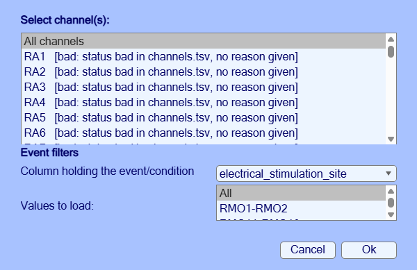
EEG = ieeglab_load(EEG, struct('event_field', 'electrical_stimulation_site'));iEEGLAB > Preprocess iEEG data, with the settings of the authors' code:
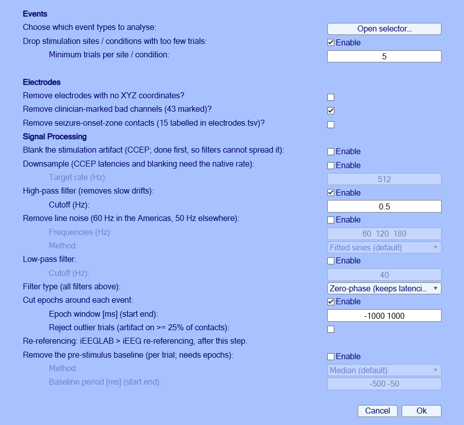
- Choose which event types to analyse: Open selector, RMO8-RMO9.
- Untick Remove electrodes with no XYZ coordinates: RP18 and ROC14 are good contacts, and the authors keep them.
- Untick Blank the stimulation artifact.
- Tick High-pass filter, cutoff 0.5 Hz.
- Untick Remove line noise: CARLA removes it from its own copy of the data before it ranks the channels, as the authors' code does; the re-referenced data keep it. That step needs the Signal Processing Toolbox: without it, CARLA ranks the channels with the line noise in (iEEGLAB > Check installation lists the toolbox).
- Untick Remove the pre-stimulus baseline.
- Keep the rest: bad contacts removed, epochs -1 to 1 s.
Expect. About 20 seconds: 212 contacts, 12 epochs.
Note. The authors high-pass with a Butterworth filter, iEEGLAB with a FIR filter (both zero-phase). The channels chosen at step 4 are the same.
EEG = ieeglab_preprocess(EEG, struct('event_filters', struct('type', {{'RMO8-RMO9'}}), ...
    'remove_no_coords', false, 'remove_bad_channels', true, 'apply_blank', false, ...
    'apply_highpass', true, 'highpass', 0.5, 'apply_notch', false, ...
    'apply_epoch', true, 'epoch_window', [-1000 1000], 'reject_trials', false, 'apply_baseline', false));
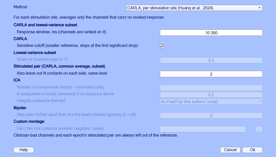
EEGpre = EEG; % kept for step 6iEEGLAB > iEEG re-referencing: CARLA, defaults. They are the authors' settings for real data: a response window of 10 to 300 ms, the sensitive cutoff, and the stimulated pair with 2 contacts on each side of it left out, as the bad contacts.
Expect. About 10 seconds. The command window reads 154/212 channels in reference, 6 excluded (RMO6 to RMO11): of the 206 channels CARLA may use, it keeps 154, the same 154 as the authors' code (Huang et al., 2024, Figure 5). The random draws use a fixed seed, so the result repeats from run to run.
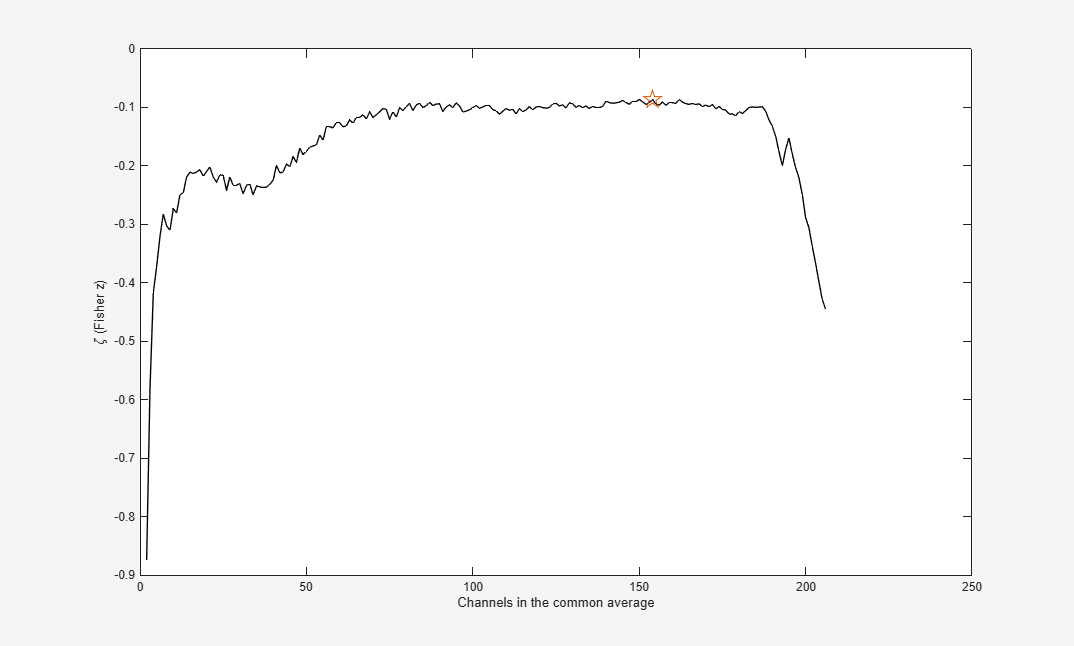
EEG = pop_ieeglab_reref(EEG, 'method', 'carla');From the command line. CARLA ranks the channels by their covariance across trials, lowest first, and adds them to the common average one at a time. For each number of channels, it re-references the data with that average and finds the channel of the average most anticorrelated with the re-referenced channels: a channel that carries a response becomes anticorrelated with the others once its response is in the average. The curve is that channel's correlation (Fisher z, the paper's zeta), averaged over 100 bootstrap draws of the trials. CARLA keeps the number of channels at the top of the curve, before the first significant drop (the sensitive cutoff).
Expect. The curve starts at -0.87 with 2 channels (1 channel has no value), rises to a plateau near -0.1 from about 80 to 180 channels, peaks at -0.086 with 154 channels (the star), and falls to -0.29 with 200 channels and -0.45 with all 206: the channels ranked last carry the response.
S = EEG.ieeglab.car.groups(1).stats;   % CARLA's statistics for the site
z = mean(S.zMinMean, 2);                % one value per number of channels: mean of the 100 draws
n = numel(S.chsUsed);                   % the number chosen
figure; plot(z, 'k'); hold on; plot(n, z(n), 'p', 'MarkerSize', 14)
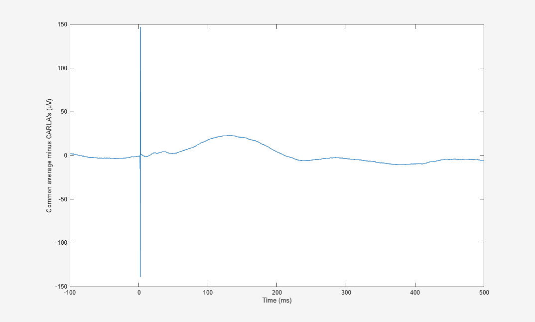
xlabel('Channels in the common average'); ylabel('\zeta (Fisher z)')In EEGLAB's Datasets menu, select the dataset that preprocessing made (before CARLA). Then iEEGLAB > iEEG re-referencing: Common average (all good channels), with 2 in Also leave out N contacts on each side, so that both averages leave out the same contacts.
Expect. 206 channels in the common average. Between 10 and 300 ms, its trial mean differs from CARLA's by up to 23 µV, 134 ms after the pulse: the responses of the 52 channels that CARLA leaves out.
EEGcar = pop_ieeglab_reref(EEGpre, 'method', 'car', 'neighbors', 2);
% the two common averages, trial mean
G = EEG.ieeglab.car.groups(1); Gc = EEGcar.ieeglab.car.groups(1);
avg = @(labels) mean(mean(EEGpre.data(ismember({EEGpre.chanlocs.labels}, labels), :, :), 3), 1);
figure; plot(EEGpre.times, avg(Gc.reference) - avg(G.reference)); xlim([-100 500])
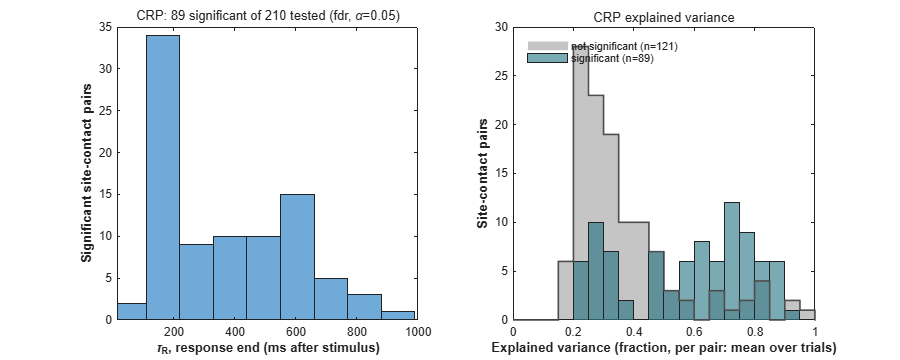
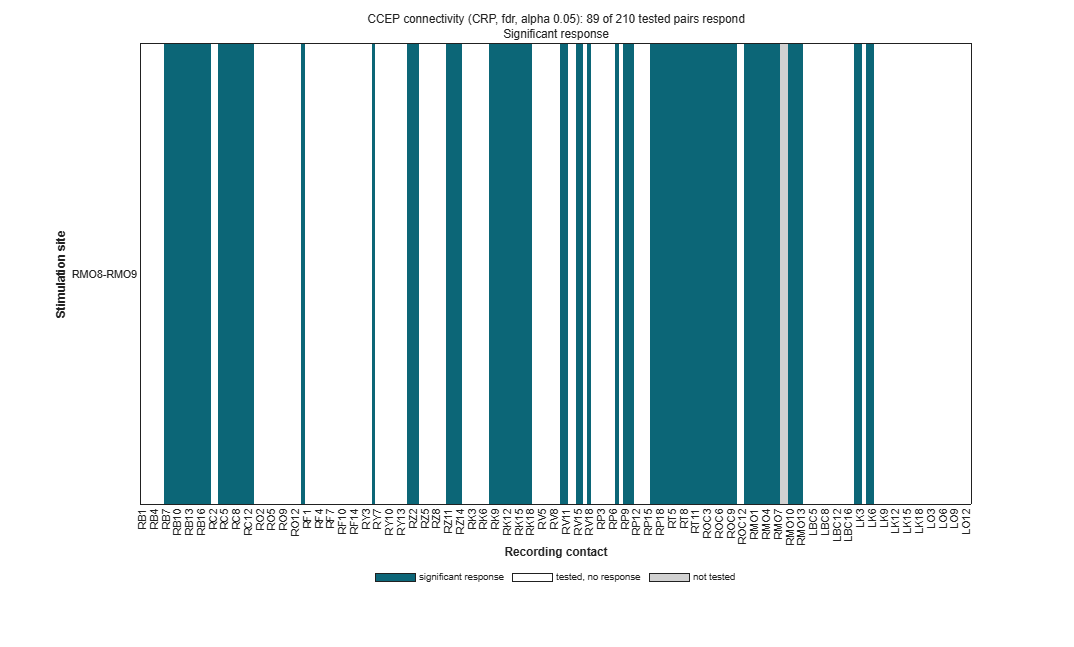
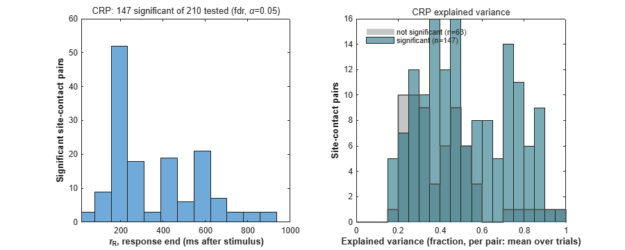
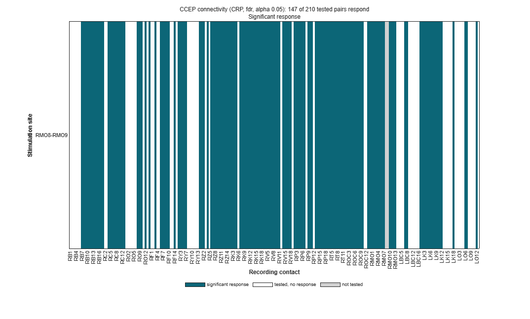
xlabel('Time (ms)'); ylabel('Common average minus CARLA''s (uV)')iEEGLAB > CCEP analysis, defaults, once on the CARLA dataset and once on the common average dataset (select each in the Datasets menu). The response of each contact is described by the Canonical Response Parameterization (CRP; Miller et al., 2023), with a permutation test.
Expect. A few seconds each. After CARLA, 89 of the 210 contacts respond; after the common average, 147 do. The common average subtracts the responses it carries from every contact, which can make contacts without a response of their own look responsive (Huang et al., 2024).
opt = struct('run_n1', false, 'run_crp', true, 'run_matrix', true, 'matrix_source', 'crp');
EEG = ieeglab_stats_subject(EEG, opt);
EEGcar = ieeglab_stats_subject(EEGcar, opt);If a result differs from Expect, a step fails, or a window is unclear, please open an issue with the message and the MATLAB command window, and the MATLAB and EEGLAB versions and operating system.
- Huang, H., Ojeda Valencia, G., Gregg, N. M., Osman, G. M., Montoya, M. N., Worrell, G. A., Miller, K. J., & Hermes, D. (2024). CARLA: Adjusted common average referencing for cortico-cortical evoked potential data. Journal of Neuroscience Methods, 407, 110153.
- Miller, K. J., Müller, K.-R., Ojeda Valencia, G., Huang, H., Gregg, N. M., Worrell, G. A., & Hermes, D. (2023). Canonical response parameterization: Quantifying the structure of responses to single-pulse intracranial electrical brain stimulation. PLOS Computational Biology, 19(5), e1011105.