Repository navigation
3 FieldTrip tutorial data
FieldTrip's intracranial tutorial data (SubjectUCI29; Stolk et al., 2018): 26 epochs with two ECoG grids and seven depth leads. The same analysis as the FieldTrip tutorial, through the iEEGLAB menus: common average of the grids, bipolar depth leads, time-frequency power and high-frequency activity, plus a test of each contact against its baseline. No stimulation here: these steps work on any epoched iEEG data.
Install iEEGLAB first (Installation). FieldTrip itself is not needed.
Four files from FieldTrip's download server, about 205 MB, kept in this folder structure, and a fifth for the comparison with FieldTrip (Against FieldTrip):
- SubjectUCI29_data.mat (the epochs, 197 MB)
- SubjectUCI29_elec_acpc_f.mat (contact positions)
-
freesurfer/surf/: lh.pial and rh.pial (the participant's brain) - SubjectUCI29_freq.mat (FieldTrip's result of the tutorial, 5 MB; for the comparison only)
iEEGLAB > Import FieldTrip epochs (.mat): select SubjectUCI29_data.mat. In the next window, Electrode
positions: SubjectUCI29_elec_acpc_f.mat; Channel types: LPG* ECOG; LTG* ECOG; * SEEG; keep the event type.
Expect. A few seconds: 152 channels at 5000 Hz, 96 ECoG (grids LPG and LTG) and 56 sEEG, 26 epochs from -400 to 900 ms, every contact with a position (ACPC space). A warning: the positions file gives the unit as volts, but the values are microvolts; they are kept as they are.
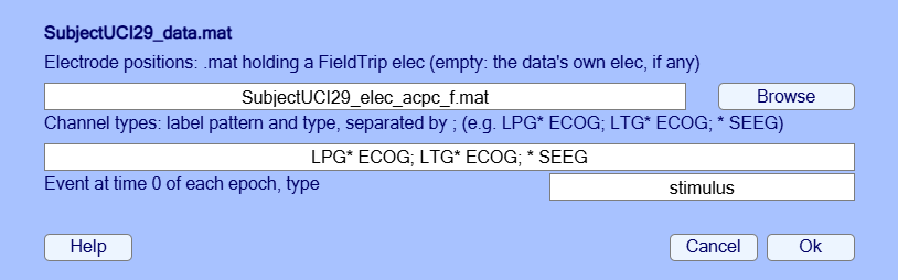
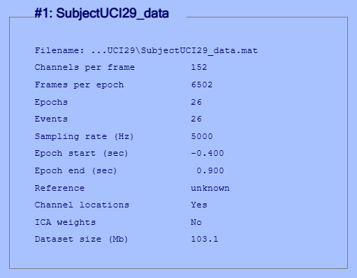
EEG = ieeglab_import_fieldtrip('SubjectUCI29_data.mat', 'elec', 'SubjectUCI29_elec_acpc_f.mat', ...
'types', {'LPG*', 'ECOG'; 'LTG*', 'ECOG'; '*', 'SEEG'});iEEGLAB > Choose brain surfaces: Select pial files, then lh.pial and rh.pial together, in freesurfer/surf.
Then iEEGLAB > Visualize electrodes.
Expect. The command window: every brain figure of this dataset is drawn on lh.pial and rh.pial. The two grids over the left hemisphere, and depth leads in both: LAM, LHH and LTH on the left, RAM, RHH, ROC and RTH on the right. A template brain would not line up: the positions are in this participant's space. A warning says that 22 of the 152 contacts lie outside the surfaces: all are grid contacts, 0.8 to 9 mm outside (3.5 mm in the median). The grids rest on the cortex, and these positions are not yet corrected for the brain shift after implantation (FieldTrip's tutorial corrects them later, in
SubjectUCI29_elec_acpc_fr.mat). Every depth contact is inside: the spaces do match.
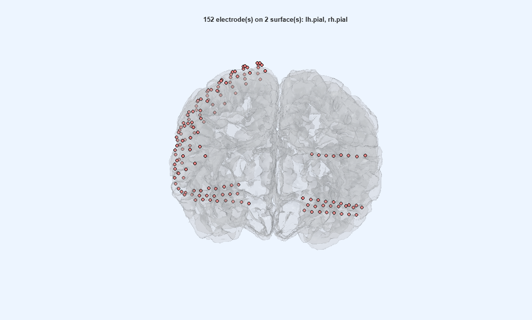
EEG = pop_ieeglab_surfaces(EEG, 'surf_files', {fullfile('freesurfer', 'surf', 'lh.pial'), ...
    fullfile('freesurfer', 'surf', 'rh.pial')});
EEG = ieeglab_vis_elec(EEG);
EEGall = EEG; % all 152 channels, for the depth leadsEdit > Select data: Channel type(s) ECOG, Ok, and keep the result as a new dataset.
Expect. 96 channels, 26 epochs.
EEG = pop_select(EEGall, 'chantype', {'ECOG'});iEEGLAB > iEEG re-referencing: choose Common average in Method.
Expect. As in the FieldTrip tutorial: the average of the 96 grid contacts is taken out of each of them.
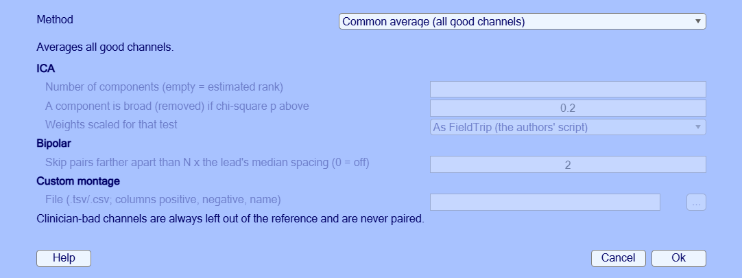
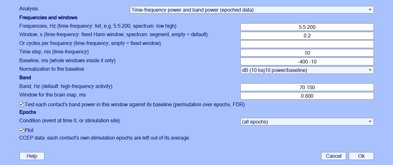
EEG = pop_ieeglab_reref(EEG, 'method', 'car');iEEGLAB > Frequency analysis: Time-frequency power and band power. Baseline -400 -10 and Window for the
brain map 0 800, as in the FieldTrip tutorial; tick Test each contact's band power in this window against its
baseline; keep the rest (5 to 200 Hz, Hann windows of 0.2 s, dB, 70-150 Hz).
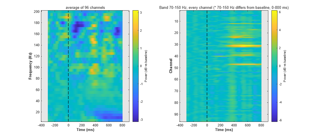
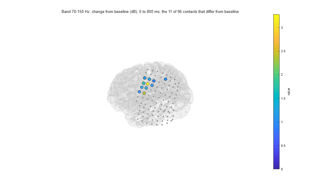
Expect. Two figures, as on the sEEG page (step 12). The times from -400 to -310 ms and from 810 to 900 ms are grey: a 0.2 s window centred there would run past the epoch. 11 of 96 contacts increase their 70-150 Hz power from baseline, all on LPG: most LPG31 (+3.3 dB), LPG47 (+2.4 dB) and LPG32 (+1.8 dB), then LPG39, LPG23, LPG40, LPG24, LPG30, LPG12, LPG48 and LPG22 (+0.9 to +1.3 dB). None decreases; the smallest corrected p among the others is 0.065. The average of the contacts rises most at 145 Hz, 390 ms (+2.3 dB). The brain map repeats the surface warning of step 2, for the same 22 grid contacts (23% of the 96).
EEG = pop_ieeglab_spectral(EEG, 'type', 'timefreq', 'baseline', [-400 -10], 'band_window', [0 800], 'stats', true);In the Datasets menu, go back to the dataset with all 152 channels, the one made by Choose brain surfaces. Then
Edit > Select data: Channel type(s) SEEG, Ok, and keep the result as a new dataset.
Expect. 56 channels, 26 epochs.
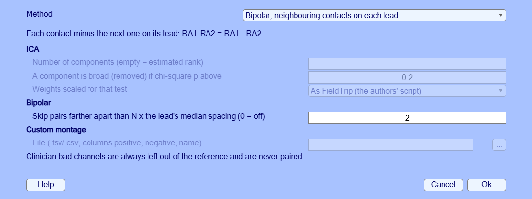
EEG = pop_select(EEGall, 'chantype', {'SEEG'});iEEGLAB > iEEG re-referencing: choose Bipolar in Method, keep the default.
Expect. Each contact minus the next one on its lead: 56 contacts become 49 channels (seven leads of eight contacts), none left out.
EEG = pop_ieeglab_reref(EEG, 'method', 'bipolar');iEEGLAB > Frequency analysis: the same as for the grids (baseline -400 -10, brain map 0 800, test ticked).
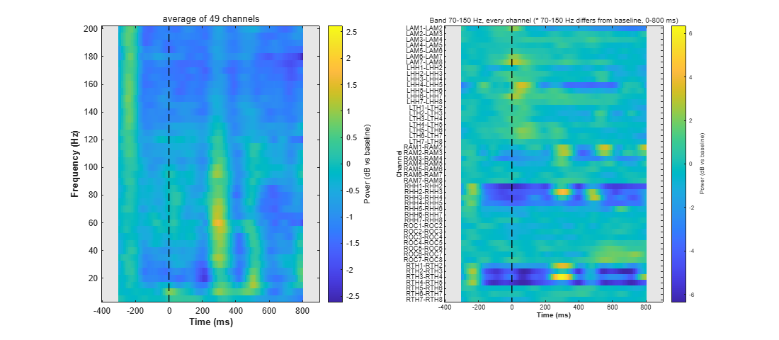
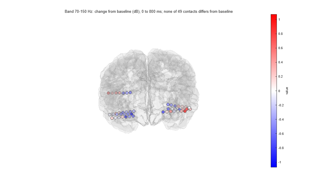
Expect. No channel differs from its baseline (smallest corrected p 0.86). The 70-150 Hz power over 0 to 800 ms goes from -4.7 dB (RTH4-RTH5) to +0.8 dB (ROC7-ROC8): a large value with no difference comes from a few epochs, as the map shows the change of the mean power and the test each epoch's change. The average of the channels rises most at 60 Hz, 300 ms (+1.6 dB).
EEG = pop_ieeglab_spectral(EEG, 'type', 'timefreq', 'baseline', [-400 -10], 'band_window', [0 800], 'stats', true);The same steps in FieldTrip (common average of the grids and bipolar depth leads with ft_preprocessing, then
ft_freqanalysis with Hann windows of 0.2 s at 5 to 200 Hz every 10 ms, as the tutorial) give the same 145 channels
and the same power: time-frequency r = 0.999997 (largest difference 0.03 in relative change), 70-150 Hz activity
r = 1.0000, and the same ten strongest channels. The tutorial has no statistics; the test above is iEEGLAB's. The
comparison reads FieldTrip's result from SubjectUCI29_freq.mat, so FieldTrip itself is not needed; it takes about
10 s.
addpath(fullfile(fileparts(which('eegplugin_ieeglab')), 'validation'));
out = validate_fieldtrip_uci29(pwd); % the folder with the three .mat filesIf a result differs from Expect, a step fails, or a window is unclear, please open an issue with the message and the MATLAB command window, and the MATLAB and EEGLAB versions and operating system.
- Stolk, A., Griffin, S., van der Meij, R., Dewar, C., Saez, I., Lin, J. J., Piantoni, G., Schoffelen, J.-M., Knight, R. T., & Oostenveld, R. (2018). Integrated analysis of anatomical and electrophysiological human intracranial data. Nature Protocols, 13(7), 1699-1723.