We have the following problem:
A company has a fleet of devices transmitting daily aggregated telemetry attributes. Predictive maintenance techniques are designed to help determine the condition of in-service equipments in order to predict when maintenance should be performed. This approach promises cost savings over routine or time-based preventive maintenance, because tasks are performed only when warranted.
For more analysis and code, please check out the Jupyter notebook.
- From the dataset, we will build a model that will determine whether a device needs maintenance utilizing Machine Learning techinuqes.
- To do this, we will apply sampling methods to an imbalanced dataset and create in-depth data exploratory analysis to understand features
- Our goal is to not only to have optimal metrics, but also minimize false negatives as much as possible
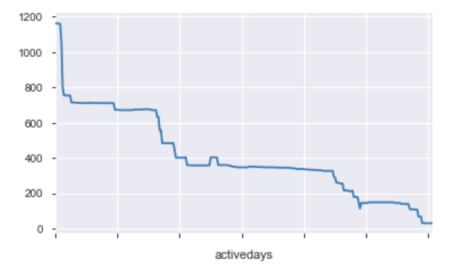
The graph below represents the amount of devices that are checked day by day. From the visualization, we can see that as each day passes, there are fewer devices that are being checked. There is a notable drop in devices checked in the beginning. All of the data recorded is within one year from 11/02/2015 to 01/01/2015.
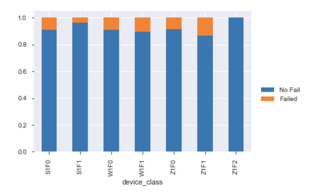
There are 7 different types of devices. Below is the visualization of how often a device fails for each class.
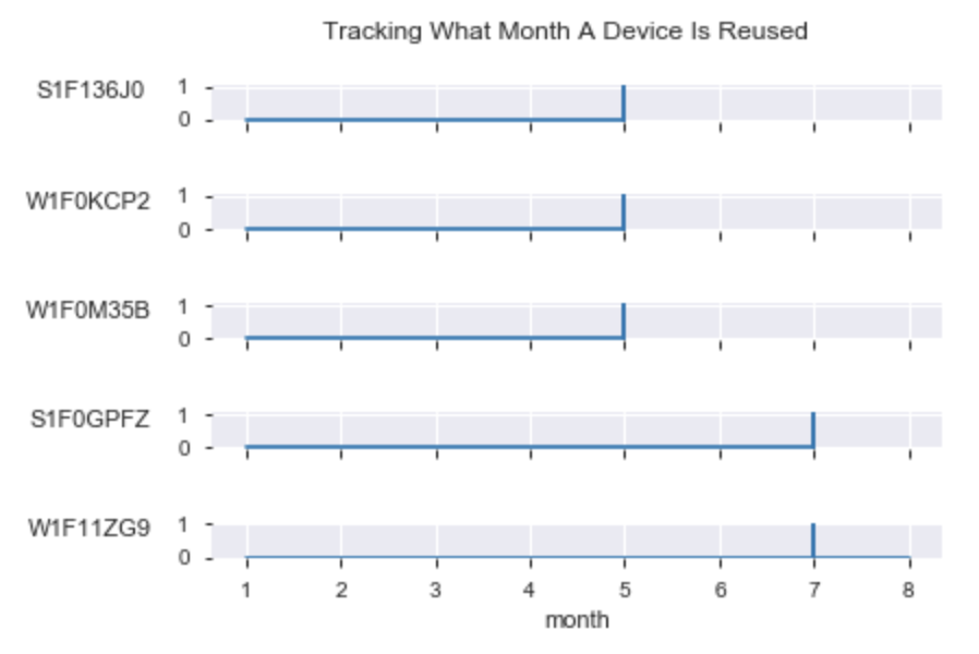
Most devices that fail are not reused. However, there are certain cases where a device is actually fixed and then resused for the future. There are a total of 5 cases below.

-
The dataset is clean, and there are no missing values. All values are integer type. There is no need to fill in values.
-
The dataset is imbalanced, about 0.1% of the classes are failures. We will need to be deal with this problem by either upsampling or downsampling.
-
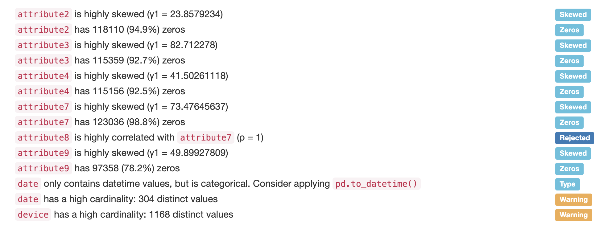
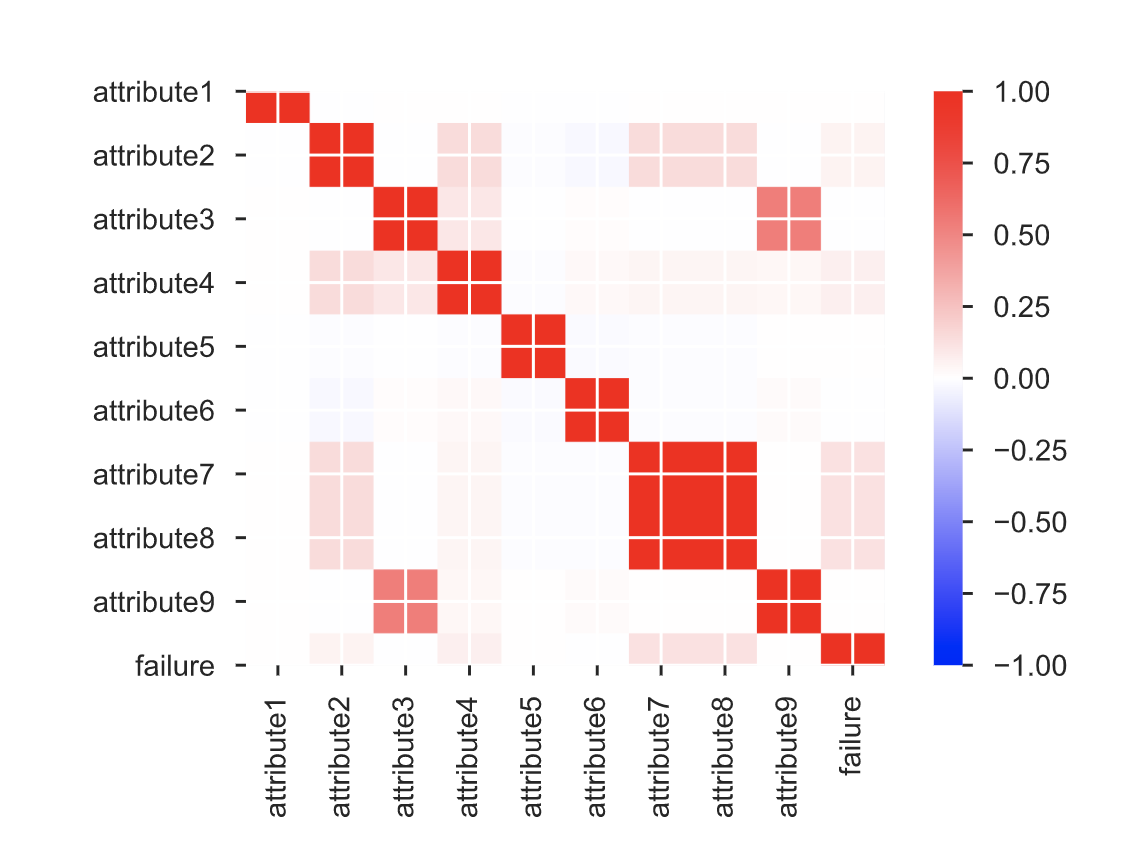
The sparse number of distinctive values in numerous columns most likely represents categorical variables. These attributes are attribute 3, 5, 7, 9, which I will encode for modeling purposes.
-
Attribute 7 and 8 are the same, so we will drop one of the two columns.
-
Attribute 2, 3, 4, 5, 7, 9 are highly skewed. We will need to apply transformations. The magnitudes differ by a wide margin. Therefore scaling needs to be done. I used min max scaler to normalize the feature from range 0 to 1 and to keep the outliers.
In our dataset, the majority of the results do not fail. As mentioned above, only about 0.1% of the classes are failures. Because we have a scarcity of data, we will choose to oversample on the failure to provide more data for modeling. We have to be careful to split the dataset first and then oversample because we do not want to duplicate observations from the train set into the test set to avoid overfitting or memorization of data points.
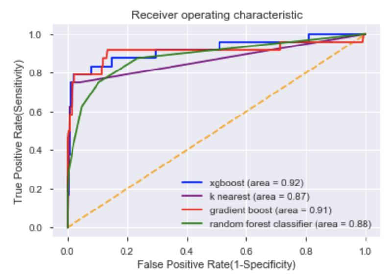
The Receiver Operating Characteristic Curve compares the true positive rate versus the false positive rate. I have ran several models and plotted their ROC curve to determine which model provides the best combination of TPR and FPR based on the largest area under the curve (AUC). The XGBoost Model with an area of 0.92 provided the best result.
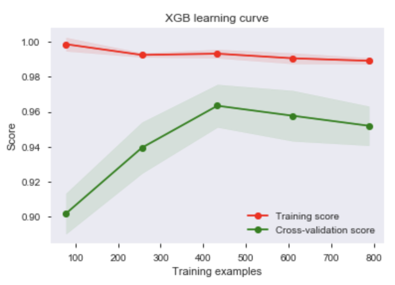
The learning curve determines whether the models needs more samples to improve its score. The colored range surrounding the lines represents the amount of variance error.
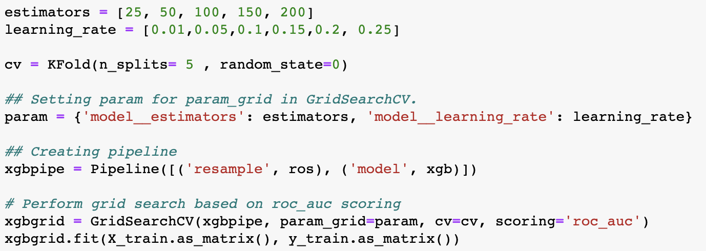
To improve our model's score, we will perform a grid search to find the best combination of parameters. Cross validation is used to allow more data to be used for model to learn and decide the parameters.
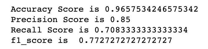
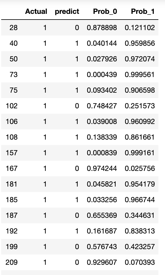
We were able to create a model that solves our overfitting problem. While we were able to predict very highly in accuracy and precision, the recall score and f1 score is slightly lower. These scores may be improved if we have more information about the attributes. Time series analysis may be applied as well to analyze what caused the dip in checking devices in the first few days.