CC-Pan: Channel-wise Compression based Diffusion
for Efficient Pan-Sharpening

Junjie Li · Congyang Ou · Haokui Zhang · Guoting Wei · Shengqin Jiang · Ying Li

Given a PAN–LRMS image pair, CC-Pan fine-tunes a pre-trained diffusion model to generate a HRMS image.

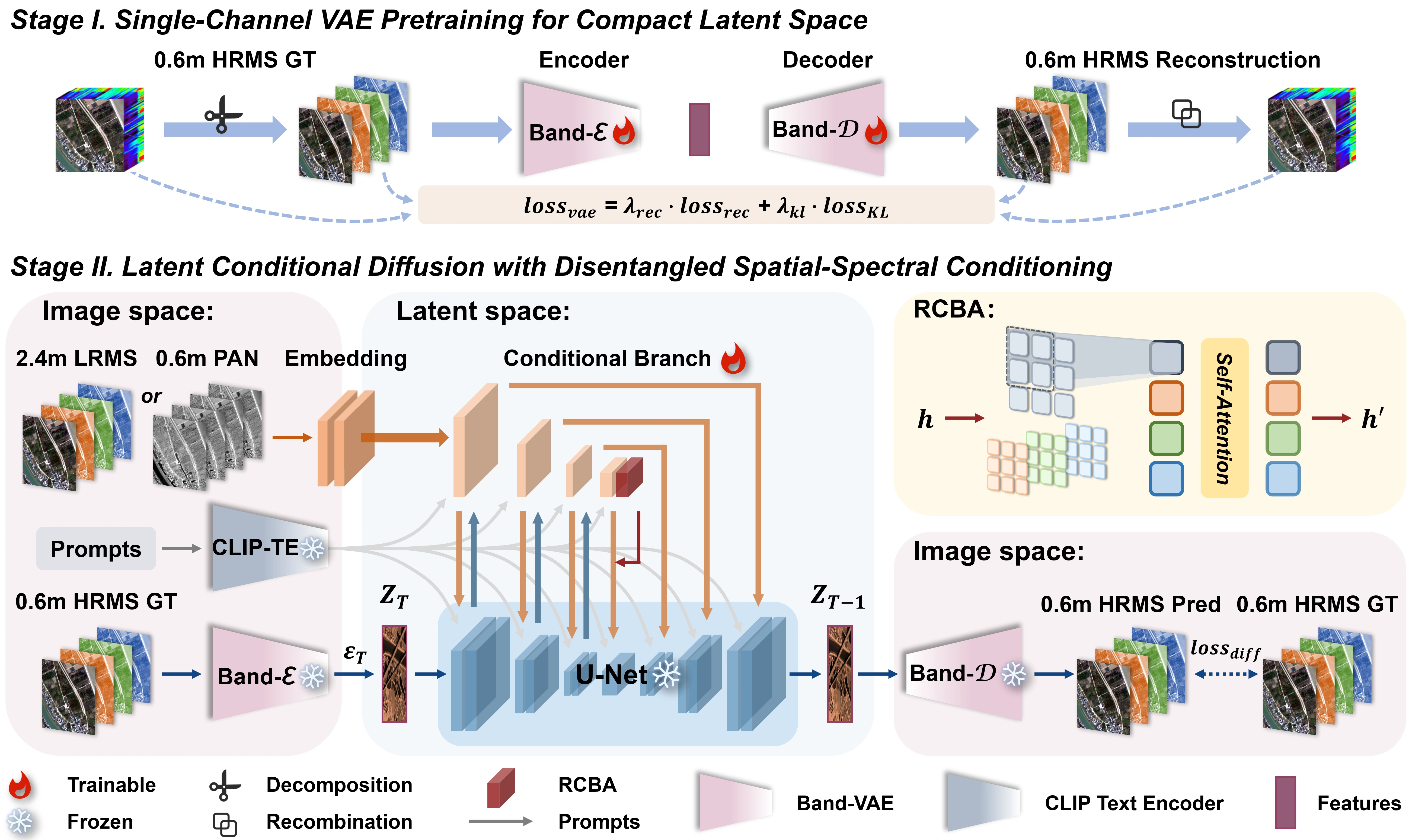
CC-Pan is a diffusion-based pan-sharpening framework that compresses multispectral channels into a compact latent space and reconstructs high-resolution multispectral imagery with a lightweight dual-branch adapter. This repository includes the training pipeline, offline inference entry points, checkpoint layout, and the Gradio demo used to reproduce the paper workflow.

News

• [02/01/2026] Code will be released soon!

At a Glance

• Task: pan-sharpening from a PAN image and a low-resolution multispectral image.
• Training stages: a 1-channel Band-VAE pretraining stage followed by latent diffusion + adapter tuning.
• Main entry points: train_vae.py, train_diffusion.py, inference.py, and app.py.
• Local assets: the repository expects local base-model files, checkpoints, and H5 datasets under the documented directory layout.

Contents

• At a Glance
• Quick Start
• Setup
• Usage
• Demo
• Repository Layout
• Results
• Reproducibility
• FAQ
• Contributing
• Maintenance
• License
• Citation
• Shoutouts

Quick Start

1. Clone the repository and install the editable local diffusers package.
2. Download the Stable Diffusion base model together with the CC-Pan VAE and adapter checkpoints.
3. Prepare PanCollection-style H5 datasets and point your YAML configs to those local paths.
4. Launch Stage-I VAE training, then Stage-II diffusion training, and finally run inference.py for evaluation.

Setup

Requirements

Before installation, make sure you have:

• Git access for cloning the repository.
• A Conda environment with Python 3.10 available locally.
• A CUDA-capable PyTorch runtime that matches your GPU driver.
• Enough local disk space for the Stable Diffusion base model, training checkpoints, and H5 datasets.

git clone https://github.com/JJLibra/CC-Pan.git
cd CC-Pan

conda create -n ccpan python=3.10 -y
conda activate ccpan

# This project depends on a modified local version of `diffusers` under `./diffusers`.
cd diffusers
pip install -e .

cd ..
pip install -r requirements.txt

If you plan to train or evaluate on GPU, installing an xformers build compatible with your local PyTorch/CUDA stack is recommended for better memory efficiency.

Initialize an 🤗 Accelerate environment with:

accelerate config

Or use a default Accelerate configuration without answering environment questions:

accelerate config default

For single-GPU runs, review configs/accelerate.yaml and adjust fields such as gpu_ids, num_processes, and mixed_precision to match your machine.

Weights

We provide two-stage checkpoints:

• Stage I (Band-VAE): checkpoints/vae.safetensors Download: Hugging Face

• Stage II (Latent Diffusion): runs on top of Stable Diffusion in the Band-VAE latent space.

  • Stable Diffusion base: download from Hugging Face (e.g., Stable Diffusion v1-5)
  • Adapters: checkpoints/adapters.pth Download: Hugging Face

Expected local layout after downloading:

base/
  stable-diffusion-v1-5/
checkpoints/
  vae.safetensors
  adapters.pth

Datasets

Dataset preparation details are documented in data/README.md. The training and evaluation pipeline expects PanCollection-style H5 files for sensors such as GF2, QB, and WV3, plus the merged data/vae/train_gt_1ch_all.h5 file used by Stage-I VAE training.

Repository Layout

• train_vae.py: Stage-I Band-VAE training entry point.
• train_diffusion.py: Stage-II diffusion + adapter training entry point.
• inference.py: offline inference and evaluation script for H5 datasets.
• app.py: Gradio demo for interactive experimentation.
• configs/: training and inference YAML configurations.
• core/: project model components and diffusion pipeline implementation.
• utils/: data prep and metric utilities.
• scripts/: convenience shell launchers.
• data/: dataset root and expected structure notes.
• checkpoints/: local checkpoint storage.
• base/stable-diffusion-v1-5/: local SD v1.5 base model files.

Usage

Before launching experiments, double-check that your YAML files point to the correct base model directory, checkpoint files, dataset H5 files, and output directory.

All main scripts also accept repeated -o key=value overrides, which is useful for changing a few paths or runtime options without duplicating full YAML files.

Training

We train the model in two stages.

Pass your dataset- and path-specific YAML file through --config for both stages.

• Stage I (VAE pretraining)

accelerate launch --config_file configs/accelerate.yaml train_vae.py --config <path/to/train_vae.yaml>

• Stage II (Diffusion + Adapter training)

accelerate launch --config_file configs/accelerate.yaml train_diffusion.py --config <path/to/train_diffusion.yaml>

If you prefer shell wrappers, scripts/train_vae.sh and scripts/train_diffusion.sh mirror the same two-stage workflow.

Note: Training usually takes 40k–50k steps, which is about 1–2 days on eight RTX 4090 GPUs in fp16. Reduce batch_size if your GPU memory is limited.

In practice, Stage-I validation is often organized around GF2/QB/WV3 splits, while Stage-II can consume multiple training and validation H5 files through list-style YAML entries.

Inference

Once training is finished, run inference:

python inference.py --config <path/to/inference.yaml>

Common inference fields to review are input_h5_paths, input_h5_names, inference_count, save_pred_h5, save_visual_rgb, and save_metrics_jsonl.

For custom experiments or notebook-style integration, the core pipeline can also be loaded directly in Python:

import torch
from diffusers import AutoencoderKL, DDPMScheduler, UNet2DConditionModel, UniPCMultistepScheduler
from transformers import AutoTokenizer, CLIPTextModel
from core.components.cc_pan import DualBranchXSAdapter, UNetDualBranchXSModel
from core.pipelines.cc_pan import StableDiffusionDualBranchXSPipeline

device = "cuda"
dtype = torch.float16

base_model = "base/stable-diffusion-v1-5"
vae_path = "output/vae_c1_gf2_qb_wv3"
adapter_weights = "output/diffusion_model/dual_branch_xs_adapter.pt"

tokenizer = AutoTokenizer.from_pretrained(base_model, subfolder="tokenizer", use_fast=False, local_files_only=True)
text_encoder = CLIPTextModel.from_pretrained(base_model, subfolder="text_encoder", local_files_only=True)
vae = AutoencoderKL.from_pretrained(vae_path, local_files_only=True)
base_unet = UNet2DConditionModel.from_pretrained(base_model, subfolder="unet", local_files_only=True)

adapter = DualBranchXSAdapter.from_unet(base_unet, size_ratio=0.25, conditioning_channels=5, conditioning_channel_order="rgb")
unet = UNetDualBranchXSModel.from_unet(base_unet, adapter=adapter)
unet.load_state_dict(torch.load(adapter_weights, map_location="cpu"), strict=False)

scheduler = UniPCMultistepScheduler.from_config(
    DDPMScheduler.from_pretrained(base_model, subfolder="scheduler", local_files_only=True).config
)

pipe = StableDiffusionDualBranchXSPipeline(
    vae=vae,
    text_encoder=text_encoder,
    tokenizer=tokenizer,
    unet=unet,
    adapter=None,
    scheduler=scheduler,
    safety_checker=None,
    feature_extractor=None,
    requires_safety_checker=False,
).to(device)

prompt = ["GaoFen-2 satellite Band Red 630-690nm"]
conditioning = torch.randn(1, 5, 128, 128, device=device, dtype=dtype)  # replace with real [LR*4, PAN]

image = pipe(
    prompt=prompt,
    image=conditioning,
    num_inference_steps=20,
    guidance_scale=1.0,
    conditioning_scale_spa=1.0,
    conditioning_scale_spe=1.0,
    output_type="pil",
).images[0]

image.save("cc_pan_demo.png")

In real use, replace the random conditioning tensor with the aligned LRMS/PAN input pair and adapt the text prompt to the target sensor or band description used by your config.

Installing xformers is highly recommended for better GPU efficiency and speed. To enable it, set enable_xformers_memory_efficient_attention=True.

Depending on your inference config, inference.py can save predicted H5 files, RGB previews, and per-sample metric logs, which makes it suitable for both benchmarking and qualitative inspection.

Demo

To launch the interactive Gradio demo locally:

python app.py

Make sure the demo points to valid local checkpoints and dataset paths before opening it in a browser.

Results

🚨 We strongly recommend visiting our project website for a better reading experience.

The tables below summarize reduced-resolution benchmarks across WV3, QB, and GF2, while the figures highlight both reduced- and full-resolution visual comparisons.

Quantitative Results

Table 1. Quantitative results on the WorldView-3 (WV3) dataset. Best results are in bold.

Models	Pub/Year	Q8 ↑	SAM ↓	ERGAS ↓	SCC ↑	Dλ ↓	Ds ↓	HQNR ↑
PaNNet	ICCV’17	0.891±0.045	3.613±0.787	2.664±0.347	0.943±0.018	0.017±0.008	0.047±0.014	0.937±0.015
FusionNet	TGRS’20	0.904±0.092	3.324±0.411	2.465±0.603	0.958±0.023	0.024±0.011	0.036±0.016	0.940±0.019
LAGConv	AAAI’22	0.910±0.114	3.104±1.119	2.300±0.911	0.980±0.043	0.036±0.009	0.032±0.016	0.934±0.011
BiMPAN	ACMM’23	0.915±0.087	2.984±0.601	2.257±0.552	0.984±0.005	0.017±0.019	0.035±0.015	0.949±0.026
ARConv	CVPR’25	0.916±0.083	2.858±0.590	2.117±0.528	0.989±0.014	0.014±0.006	0.030±0.007	0.958±0.010
WFANET	AAAI’25	0.917±0.088	2.855±0.618	2.095±0.422	0.989±0.011	0.012±0.007	0.031±0.009	0.957±0.010
PanDiff	TGRS’23	0.898±0.090	3.297±0.235	2.467±0.166	0.980±0.019	0.027±0.108	0.054±0.047	0.920±0.077
SSDiff	NeurIPS’24	0.915±0.086	2.843±0.529	2.106±0.416	0.986±0.004	0.013±0.005	0.031±0.003	0.956±0.016
SGDiff	CVPR’25	0.921±0.082	2.771±0.511	2.044±0.449	0.987±0.009	0.012±0.005	0.027±0.003	0.960±0.006
CC‑Pan	Ours	0.924±0.064	2.689±0.135	1.839±0.211	0.989±0.007	0.010±0.008	0.021±0.004	0.965±0.007

Table 2. Quantitative results on the QuickBird (QB) dataset. Best results are in bold.

Models	Pub/Year	Q4 ↑	SAM ↓	ERGAS ↓	SCC ↑	Dλ ↓	Ds ↓	HQNR ↑
PaNNet	ICCV’17	0.885±0.118	5.791±0.995	5.863±0.413	0.948±0.021	0.059±0.017	0.061±0.010	0.883±0.025
FusionNet	TGRS’20	0.925±0.087	4.923±0.812	4.159±0.351	0.956±0.018	0.059±0.019	0.052±0.009	0.892±0.022
LAGConv	AAAI’22	0.916±0.130	4.370±0.720	3.740±0.290	0.959±0.047	0.085±0.024	0.068±0.014	0.853±0.018
BiMPAN	ACMM’23	0.931±0.091	4.586±0.821	3.840±0.319	0.980±0.008	0.026±0.020	0.040±0.013	0.935±0.030
ARConv	CVPR’25	0.936±0.088	4.453±0.499	3.649±0.401	0.987±0.009	0.019±0.014	0.034±0.017	0.948±0.042
WFANET	AAAI’25	0.935±0.092	4.490±0.582	3.604±0.337	0.986±0.008	0.019±0.016	0.033±0.019	0.948±0.037
PanDiff	TGRS’23	0.934±0.095	4.575±0.255	3.742±0.353	0.980±0.007	0.058±0.015	0.064±0.020	0.881±0.075
SSDiff	NeurIPS’24	0.934±0.094	4.464±0.747	3.632±0.275	0.982±0.008	0.031±0.011	0.036±0.013	0.934±0.021
SGDiff	CVPR’25	0.938±0.087	4.353±0.741	3.578±0.290	0.983±0.007	0.023±0.013	0.043±0.012	0.934±0.011
CC‑Pan	Ours	0.939±0.088	4.198±0.526	3.251±0.288	0.984±0.009	0.017±0.011	0.026±0.009	0.957±0.010

Table 3. Quantitative results on the GaoFen-2 (GF2) dataset. Best results are in bold.

Models	Pub/Year	Q4 ↑	SAM ↓	ERGAS ↓	SCC ↑	Dλ ↓	Ds ↓	HQNR ↑
PaNNet	ICCV’17	0.967±0.013	0.997±0.022	0.919±0.039	0.973±0.011	0.017±0.012	0.047±0.012	0.937±0.023
FusionNet	TGRS’20	0.964±0.014	0.974±0.035	0.988±0.072	0.971±0.012	0.040±0.013	0.101±0.014	0.863±0.018
LAGConv	AAAI’22	0.970±0.011	1.080±0.023	0.910±0.045	0.977±0.006	0.033±0.013	0.079±0.013	0.891±0.021
BiMPAN	ACMM’23	0.965±0.020	0.902±0.066	0.881±0.058	0.972±0.018	0.032±0.015	0.051±0.014	0.918±0.019
ARConv	CVPR’25	0.982±0.013	0.710±0.149	0.645±0.127	0.994±0.005	0.007±0.005	0.029±0.019	0.963±0.018
WFANET	AAAI’25	0.981±0.007	0.751±0.082	0.657±0.074	0.994±0.002	0.003±0.003	0.032±0.021	0.964±0.020
PanDiff	TGRS’23	0.979±0.011	0.888±0.037	0.746±0.031	0.988±0.003	0.027±0.011	0.073±0.013	0.903±0.025
SSDiff	NeurIPS’24	0.983±0.007	0.670±0.124	0.604±0.108	0.991±0.006	0.016±0.009	0.027±0.027	0.957±0.010
SGDiff	CVPR’25	0.980±0.011	0.708±0.119	0.668±0.094	0.989±0.005	0.020±0.013	0.024±0.022	0.959±0.011
CC‑Pan	Ours	0.982±0.010	0.667±0.051	0.592±0.088	0.991±0.003	0.005±0.002	0.022±0.014	0.973±0.010

Qualitative Comparison

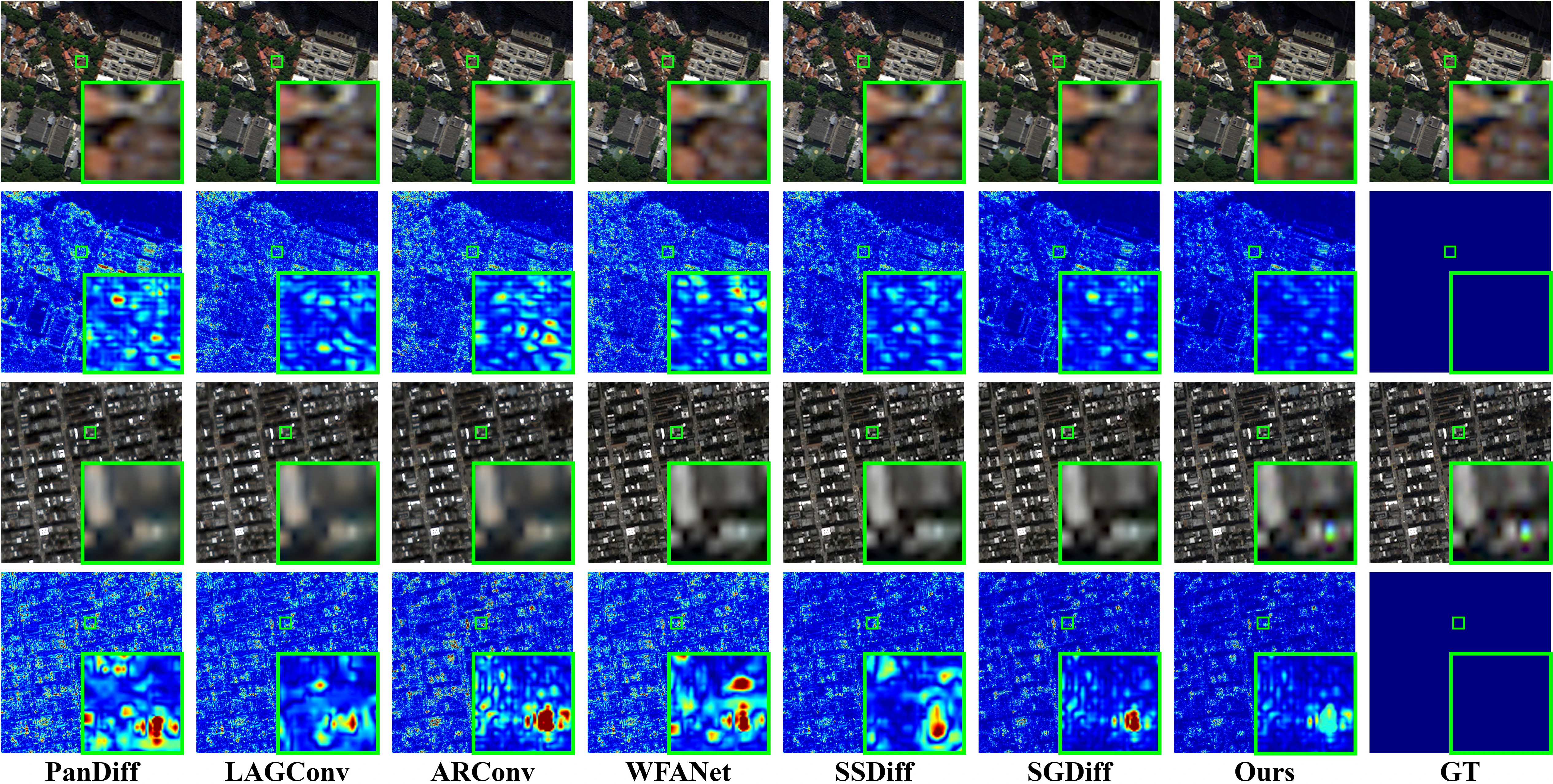
Visual comparison on the WorldView-3 (WV3) and QuickBird (QB) datasets at reduced resolution.

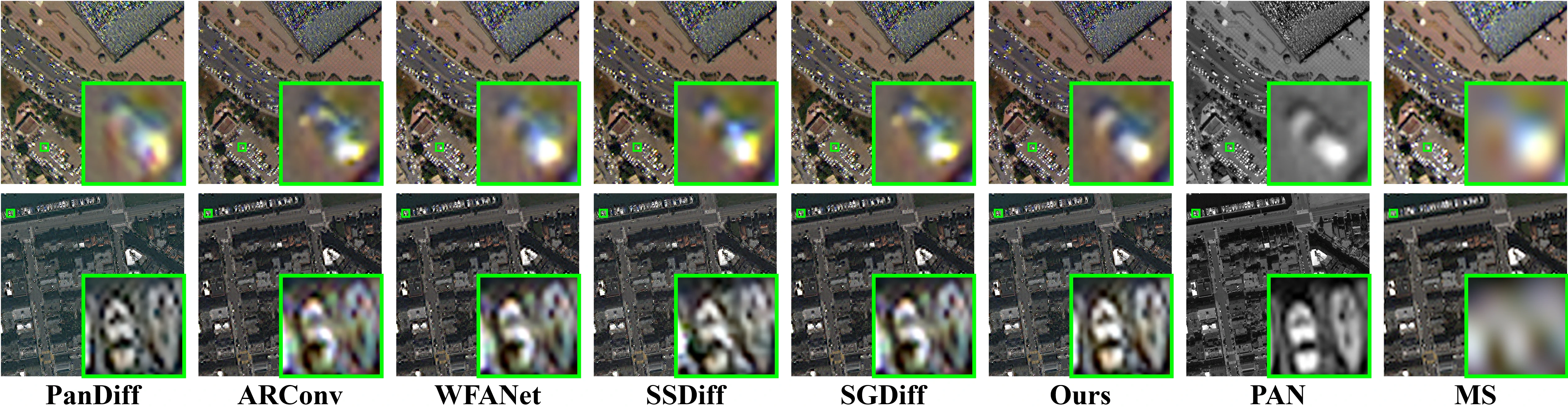
Visual comparison on the WorldView-3 (WV3) and QuickBird (QB) datasets at full resolution.

Efficiency Comparison (RR, QB)

Diffusion-based Methods	SAM ↓	ERGAS ↓	NFE	Latency (s) ↓
PanDiff	4.575±0.255	3.742±0.353	1000	356.63±1.98
SSDiff	4.464±0.747	3.632±0.275	10	10.10±0.21
SGDiff	4.353±0.741	3.578±0.290	50	6.64±0.09
CC-Pan	4.198±0.526	3.251±0.288	20	3.36±0.07

Latency is reported as mean ± std over 10 runs (warmup = 3), with batch size = 1, evaluated on the QB dataset under the reduced-resolution (RR) protocol on an RTX 4090 GPU. NFE denotes the number of function evaluations during sampling, so lower values generally correspond to faster diffusion inference.

Reproducibility

For reproducible experiments, record the exact YAML used for each stage, the accelerate launcher settings, the selected checkpoint files, and the git commit hash associated with each run.

FAQ

Do I need local Stable Diffusion weights?
Yes. The training and inference code expects a local base model directory under base/.

Why do the training commands use <path/to/...>.yaml placeholders?
Because the exact dataset paths, checkpoint locations, and output directories depend on your local setup.

What input format does offline evaluation expect?
PanCollection-style H5 files with gt, lms, and pan keys are expected by the default pipeline.

Contributing

Documentation fixes, setup clarifications, and reproducibility improvements are welcome. When preparing changes, keep paths explicit, describe any dataset assumptions, and mention whether your notes target training, inference, or the demo workflow.

Maintenance

When updating the project, keep the README in sync with checkpoint filenames, expected directory names, and any CLI arguments exposed by train_vae.py, train_diffusion.py, inference.py, or app.py.

License

This project is released under the MIT License. See LICENSE for the full text.

Citation

If you find our work useful, please cite:

@article{li2026ccpan,
  title={CC-Pan: Channel-wise Compression based Diffusion for Efficient Pan-Sharpening},
  author={Junjie Li and Congyang Ou and Haokui Zhang and Guoting Wei and Shengqin Jiang and Ying Li},
  journal={arXiv preprint arXiv:2602.04473},
  year={2026}
}

Shoutouts

• Built with 🤗 Diffusers. Thanks for open-sourcing!
• The interactive demo is powered by 🤗 Gradio. Thanks for open-sourcing!