The targeted goal of this analysis is to identify the features most associated with on-time departures. This will provide insights on how likely your next flight would be delayed based on if certain conditions are being met, such as the weather or the time of your travel to name a few.
Rationale
According to Airlines for America (A4A)in 2019, "the average cost of aircraft block (taxi plus airborne) time for U.S. passenger airlines was $74.24 per minute...Delayed aircraft are estimated to have cost the airlines several billion dollars in additional expense. Delays also drive the need for extra gates and ground personnel and impose costs on airline customers (including shippers) in the form of lost productivity, wages and goodwill." 1 In addition to the considerable losses associated with delays, there are psychological costs as well. A 2007, University of Michigan’s American Customer Satisfaction Index score for U.S. airlines registered only 63% satisfaction.2 Since the return to high volume air travel after months of pandemic-induced closed borders and the grounding of most flights, we have seen a disturbing rise in "passenger unruliness". According to a recent CNN report, the FAA has issued more than $1 million in fines to such passengers already in 2021. 3 while most of the media attention has been focused on the refusal to wear masks during flights, data from the IATA from 2012-2015 demonstrate the rise of passenger disruption well before the onset of the pandemic.4 Many reasons contribute to this rise: fuller cabins, shrinking leg space, increased security checks, additional fees for cary-on bags, etc. Such issues are endemic to the industry and effect all carriers to varying degrees. However, flight delays, as already mentioned, add to an already challenging travel sector.
Description data source
This is a classification dataset with detailed airline, weather, airport and employment information collected from the Bureau of Transportation statistics, National Center for Environment Information (NOAA). Flight delay data has been curated by Jen Wadkins and stored on kaggle.com (https://www.kaggle.com/threnjen/2019-airline-delays-and-cancellations) and includes 24 raw data files, 1 train_test_small (Jan 2019), 1 train_test 2019, new_data 2020 and new_data_small (2020). We are using 1 large train_test consisting of 6.5 million records as our universe.
Question
"What are the key features most correlated to on-time departures?"
EDA
-
Our initial dataset (train_test.csv) is a very clean and high quality file, consisting of 6,538,721 rows with no null values. Tableau was used in combination with the dataset to perform exploratory data analysis on the dataset. Key features were plotted against the number of departure delays for the year of 2020. These features were plotted to provide a high level overview of the data to assess which features were associated with the largest number of delays. Key features that were originally targeted for machine learning were: plane age in years, concurrent flights by plane, average wind speed in miles per hour, average max temperature in fahrenheit, plane segment number, airline flights per month, airport flights per month, departure block by time of day, average precipitation in inches, and average snowfall in inches.
-
Database EDA: pgAdmin postgres was also used for exploratory data analyis. Tables were created to compare aggregate measures of the previously mentioned target features in the EDA section.

Data munging will be described below and consists of removing duplications for August records.
Description of the analysis phase of the project
- Used SQL queries, Tableau and pandas notebooks to execute initial analysis, using cross tables and matplotlib charts to visualize the data.
- We used R to initially generate a sample size that our tools could properly analyze.
- It is here that we discovered that the month of September was missing and that August data was duplicated. We used python to remove duplicate records and resample the dataset to train/test in our machine learning models.
Technologies, languages, tools, and algorithms used throughout the project
- Technologies: Postgres SQL (pgAdmin), AWS, Google (Collab, Slides, Drive), Tableau (Tableau Public), Pandas Notebook
- Languages: Python, R, SQL
- Libraries: matplotlib, os, pathlib, numpy, seaborn, sklearn, collections, imblearn
GitHub
Our communication system is comprised of using GitHub, Slack, and Zoom to coordinate, contribute and commit our respective work. Each team member has made significant and frequent commits far exceeding the minimal requirements for this deliverable to their individual branches as well as to the main branch directly. We have also contributed to external platforms like Google (e.g., Drive, Collab, & Slides), Tableau Public, AWS.
Data Preprocessing
The data preprocessing process began by uploading all of the raw data tables to an AWS RDS database. A connection to the server was established using PgAdmin/Postgress and the group utilized this tool to create, delete, and manipulate the data tables. Please refer to the "Description data source" section for a complete description of the dataset.
As stated previously, the initial dataset (train_test.csv) is a very clean and high quality file, consisting of 6,538,721 rows with no null values. However, there were still some issues which had to be addressed in order to create a working table:
- The flight data for August was duplicated and entered twice, once as data for the Month of August and once again for the month of September. As the raw data for the individual months was available, the August duplicates were removed and the correct September data was added to the working table.
- It was determined during preliminary machine learning testing that the data set was too large for certain models to run effectively with the resources provided by google collab. As such the decision was made to slim down the working table data by random sampling the initial data set utilizing the following R Script. From this random sampling the working table "sample_train_test" was created.
The results of the initial data preprocessing culminated in a working table with following structure and content:
| MONTH | DAY_OF_WEEK | DEP_DEL15 | DISTANCE_GROUP | DEP_BLOCK | SEGMENT_NUMBER | CONCURRENT_FLIGHTS | NUMBER_OF_SEATS | CARRIER_NAME | AIRPORT_FLIGHTS_MONTH | AIRLINE_FLIGHTS_MONTH | AIRLINE_AIRPORT_FLIGHTS_MONTH | AVG_MONTHLY_PASS_AIRPORT | AVG_MONTHLY_PASS_AIRLINE | FLT_ATTENDANTS_PER_PASS | GROUND_SERV_PER_PASS | PLANE_AGE | DEPARTING_AIRPORT | LATITUDE | LONGITUDE | PREVIOUS_AIRPORT | PRCP | SNOW | SNWD | TMAX | AWND |
|---|---|---|---|---|---|---|---|---|---|---|---|---|---|---|---|---|---|---|---|---|---|---|---|---|---|
| 11 | 1 | FALSE | 4 | AFTERNOON | 3 | 18 | 70 | SkyWest Airlines Inc. | 2176 | 66502 | 228 | 197188 | 3472966 | 3.4E-05 | 9.9E-05 | 1 | Charleston International | 32.899 | -80.039 | Logan International | 0 | 0 | 0 | 71 | 3.36 |
| 1 | 4 | FALSE | 5 | EVENING | 4 | 24 | 230 | Frontier Airlines Inc. | 2327 | 9496 | 122 | 279230 | 1857122 | 0.00012 | 7E-06 | 2 | General Mitchell Field | 42.95 | -87.897 | San Diego International Lindbergh Fl | 0 | 0 | 0 | 27 | 6.04 |
With the initial data preprocessing complete and a working table formulated, there were still some additional data preprocessing steps to be done in Python/Google Collab before the machine learning models could be effectively executed.
- An efficient way to connect the Collab notebooks with the AWS database had to be implemented. This was addressed by installing a local version of Postgres in the Collab notebook and connecting to the database directly; after successfully connecting to the database, the working table was then imported into a pandas dataframe.
# Installing Postgress
!apt install postgresql postgresql-contrib &>log
!service postgresql start
!sudo -u postgres psql -c "CREATE USER root WITH SUPERUSER"

# setting connection to DB
%load_ext sql
%config SqlMagic.feedback=False
%config SqlMagic.autopandas=True
%sql postgresql+psycopg2://USERNAME:PASSWORDc@DBNAME.DBURL:5432/flight-delay-tables

df = %sql SELECT * FROM public.sample_train_test- As some of the columns in the working table contained items like airport names and other non-numerical values, these columns had to be encoded. In order for the results of the model to be more cohesive the team decided to custom encode the following variables:
DEP_BLOCK,CARRIER_NAME,DEPARTING_AIRPORTand our target featureDEP_DEL15. Below is a sample of some of the custom encoding code:
# Encoding "departure_block" feature
dep_block = {"EARLY_MORNING": 0,
             "MORNING": 1,
             "AFTERNOON": 2,
             "MIDDAY": 3,
             "EVENING": 4,
             "LATE_NIGHT": 5}

encoded_df = df.copy()
encoded_df['DEP_BLOCK'] = encoded_df['DEP_BLOCK'].apply(lambda x: dep_block[x])

# Encoding "CARRIER_NAME" feature
carrier_name = {"SkyWest Airlines Inc.": 1,
                "Frontier Airlines Inc.": 2,
                "American Eagle Airlines Inc.": 3,
                "Delta Air Lines Inc.": 4,
                "Alaska Airlines Inc.": 5,
                "Southwest Airlines Co.": 6,
                "American Airlines Inc.": 7,
                "Hawaiian Airlines Inc.": 8,
                "JetBlue Airways": 9,
                "Endeavor Air Inc.": 10,
                "United Air Lines Inc.": 11,
                "Spirit Air Lines": 12,
                "Allegiant Air": 13,
                "Midwest Airline, Inc.": 14,
                "Comair Inc.": 15,
                "Mesa Airlines Inc.": 16,
                "Atlantic Southeast Airlines": 17}

encoded_df['CARRIER_NAME'] = encoded_df['CARRIER_NAME'].apply(lambda x: carrier_name[x])- As testing progressed it was determined that in order to better utilize the available resources within the Collab Notebook and to achieve better model fitting performance, the data in the encoded dataframe had to be scaled. The scaling was achieved utilizing scikit-learn's standard scaler. Below is a sample of some of the standard scaling code:
# Creating StandardScaler instance
scaler = StandardScaler()

# Fitting Standard Scaller
X_scaler = scaler.fit(X_train)

# Scaling data
X_train_scaled = X_scaler.transform(X_train)
X_test_scaled = X_scaler.transform(X_test)
Feature engineering and feature selection
In the first iteration of feature engineering and selection, the data set was analyzed and 10 features were chosen arbitrarily as being most impactful. This approach was then refined in later stages of the project as it was determined that choosing features prior to model testing could lead to inherent bias and a less accurate models. As such all 26 features originally present in the data set were considered in the feature engineering and selection process.
The sample_train_test table contains 26 features so we performed a feature selection process to reduce the number of input variables for the predictive model. We used a combination of a tree-based estimator (i.e. random forests) and the correlation matrix to get an insight of the most influential features on the targeted variable ("DEP_DEL15" = Departure delays over 15 minutes). Below are the features selected based on the feature selection results:
'DEP_BLOCK' - Departure block
'SEGMENT_NUMBER' - The segment that this tail number is on for the day
'CONCURRENT_FLIGHTS' - Concurrent flights leaving from the airport in the same departure block
'AIRLINE_AIRPORT_FLIGHTS_MONTH' - Avg Flights per month for Airline AND Airport
'AIRPORT_FLIGHTS_MONTH' - Avg Airport Flights per Month
'PRCP' - Inches of precipitation for day
'TMAX' - Max temperature for day
'AWND' - Max wind speed for day
'SNOW' - Inches of snowfall for day
Training and Testing Sets
For all models the data was split into training and testing sets in a standard fashion as outlined by the relevant course modules.
- The feature sets were defined by defining an x variable, copying the encoded dataframe, and then dropping the target feature from the dataframe.
- Then the target set was defined as a y variable containing our targeted feature.
- Finally, the data was split into 2 sets - a Training set and a Testing set. See the code block below for a code example:
# Define the features set.
X = encoded_df.copy()
X = X.drop("DEP_DEL15", axis=1)
X.head()

# Define the target set.
y = encoded_df["DEP_DEL15"].ravel()
y[:5]

# Splitting into Train and Test sets.
X_train, X_test, y_train, y_test = train_test_split(X, y, random_state=78)
Model Choices & Changes
Initially it was decided that a Logistic Regression and a SVM model were to be utilized as our machine learning models. We experienced two major hurdles associated with our model choices:
- For the Logistic Regression model - Our results appeared to show that our model was overfitted and thus our model was not accurate in predicting delays.
- For the SVM Model - The resource limitations within Google Collab forced the group to drop this model choice as a viable one. After consulting with the instructional staff, scaling the data, and adjusting the kernel Collab used, the model would not fit the data even after 6+ hour runtimes.
Taking into account the two limitation mentioned above, the choice was made to utilize a K-nearest Neighbor Model and Ensemble Random Forest Model in an attempt to have more than one functional model and address the overfitting issue. Unfortunately, these models also experienced overfitting and the corresponding results pointed at our models being more suitable for predicting on-time arrivals rather delays.
Below is a more in depth look at the models utilized, their limitations, and their benefits.
- The targeted goal of this analysis is to create a machine learning algorithm that classifies whether a flight will be delayed or not, and then ranks the importance of several features by how greatly they impact the prediction model.
- Explanation: Logistic regression predicts binary outcomes, meaning that there are only two possible outcomes. In other words, a logistic regression model analyzes the available data, and when presented with a new sample, mathematically determines its probability of belonging to a class.
- Benefits: Logistic Regression is one of the simplest machine learning algorithms and is easy to implement yet provides great training efficiency in some cases. Also due to these reasons, training a model with this algorithm doesn't require high computation power.
- Limitations: Logistic Regression is a statistical analysis model that attempts to predict precise probabilistic outcomes based on independent features. On high dimensional datasets, this may lead to the model being over-fit on the training set, which means overstating the accuracy of predictions on the training set and thus the model may not be able to predict accurate results on the test set.
- Explanation: Random Forest Machine learning models sample a data set and build smaller and simpler decision trees, with each small tree being built from a random selection of the features specified. A combination of all these small trees, or weak learners, is combined to create a strong learner which has more robust decision making.
- Benefits: Random Forest models are good for data sets which may be prone to overfitting. This type of model can handle larger data sets without adversely impacting processing time and mitigates from inaccuracies due to outliers.
- Limitations: The model may become too large and thus too slow for real-time uses such as loan predictions. It can also be un-intuitive as to how features are impacting the predictions of the model.
- Explanation: The KNN is a supervised machine learning algorithm which assumes that similar things exist in close approximity so it captures the idea of similarity by calculating the distance between points on a graph.
- Benefits: The algorithm is simple and easy to implement and there's no need to build a model, tune several parameters, or make additional assumptions. It is also versatile in that it can be used for classification and regression data.
- Limitations: The algorithm gets significantly slower as the number of examples and/or predictors/independent variables increase. The model is not practical where predictions need to be made rapidly.
- Explanation: A Support Vector Machine model is similar to a logistic regression model in that is also a binary classifier, it splits the sample in to two categories; in our data set the two categories being Delayed or Not Delayed.
- Benefits: While SVM seeks to split our dataset into two categories, it does not do so as rigorously as a linear regression model. SMV allows for "soft" margins and has logic implemented which accounts for outliers and may make exceptions for them. This means some data points past the "cut off" line/point may still be sorted into the opposite classification.
- Limitations: The training/fitting time for large data sets is a large barrier, even with scaled data the processing time for large data sets can be lengthy and resource intensive.
- Explanation: Neural networks are set of algorithms that are modeled after the human brain. It contains layers of neuron layers, which perform individual computations. These computations are connected and weighted against one another until the neurons reach the final layer and returns a numerical result or an encoded categorical result.
- Benefits: Neural networks are effective at detecting complex, nonlinear relationships and have greater tolerance for messy data and can learn to ignore noisy characteristics in data.
- Limitations: The layers of neurons were too complex to dissect and understand.
Training the Models
In general, we utilized a similar approach for all of the models we tested and attempted to establish a standardized and repeatable process:- The Data is imported and preprocessed
- A feature selection process occurs
- The dataset is split into a Training and Test set
- The Data is scaled
- The model is initiated and the data is Fit
- The model is trained
- Data Validation occurs and accuracy scores, confusion matrixes, correlation reports, etc are formulated.
Below is an example of how the model is fit starting with step 3 on the list above:
# Separate the features from the target
X = encoded_df.drop(columns='DEP_DEL15')
y = encoded_df['DEP_DEL15']

# Split data into training and testing
X_train, X_test, y_train, y_test = train_test_split(X,
                                                    y,
                                                    random_state=1,
                                                    stratify=y)
X_train.shape

# Creating StandardScaler instance
scaler = StandardScaler()

# Fitting Standard Scaller
X_scaler = scaler.fit(X_train)

# Scaling data
X_train = X_scaler.transform(X_train)
X_test = X_scaler.transform(X_test)

# Instantiate KNN model classifier
classifier = KNeighborsClassifier(n_neighbors=5)

# Fitting the data
classifier.fit(X_train, y_train)

#Predictions

predictions = classifier.predict(X_test)

results_df = pd.DataFrame({'Prediction': predictions,
                           'Actual': y_test}).reset_index(drop=True)
results_df.head(20)

# Validation

# Generating a Confusion Matrix
cm = confusion_matrix(y_test, predictions)

cm_df = pd.DataFrame(cm, index=['Actual 0', 'Actual 1'], columns=['Predicted 0', 'Predicted 1'])

# Calculating the accuracy score
acc_score = accuracy_score(y_test, predictions)
</details>

corr_matrix = encoded_df.corr()

corr_matrix.style.background_gradient(cmap='coolwarm')

target = 'DEP_DEL15'
threshold = 0.015
correlation_scores = corr_matrix[(corr_matrix[target] > threshold) | (corr_matrix[target] < -threshold)][target]

correlation_scores.sort_values(ascending=False)
Classification Report Summary
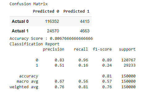
We have trained and tested the data with the following models and all of which resulted in overfitted results:
- Logistic Regression Model
- Accuracy score: 81%
- K-nearest Neighbor Model
- Accuracy score: 79%
- Ensemble Random Forest Model
- Accuracy score: 81%
- Neural Network
Database
- A fully integrated database has been created using AWS RDS and pgAdmin.
- Multiple schemas were created to store raw data files imported from csv.
- sql scripts were used to join, aggregate, transform and export data.
- Several Google Colab, Jupyter notebooks, and other scripts connect to the database to perform data cleansing, transformation, and read/write operations.
- An ERD has been provided for the raw data tables to provide a visual of the database architecture and metadata details.
Slides Presentation
Slides Presentation are drafted in Google Slides https://docs.google.com/presentation/d/18d2kpjwzPQlTeO8HySODeFJqht5v4XSi9c_GcyEFgKY/edit?usp=sharingTableau Public
https://public.tableau.com/app/profile/tommy.williams/viz/flight_delay_project/FeaturesvsAirlineDelays?publish=yesDetails
## Footnotes 1: See https://www.airlines.org/dataset/u-s-passenger-carrier-delay-costs/. 2: See https://economics.ecu.edu/wp-content/pv-uploads/sites/165/2019/07/ecu0707.pdf. 3: See https://www.cnn.com/travel/article/flight-attendants-unruly-passengers-covid/index.html. 4: Ibid.Instruction To Run the Machine Learning Models:
Follow the instruction below to successfully run one of our machine learning models. The .ipynb files with outputs have been stored in the ‘Machine Learning’ folder of the GitHub repository. Note: most of our models take anywhere from 5-10 minutes to fit.
- Navigate to the ‘Machine Learning’ portion of the GitHub repository.
- Select one of the machine learning models and download the corresponding .ipynb file. Since our highest scoring model is the “ML_ensemble_random_forest” file, we recommend running this one.
- The notebook connects to our AWS database by installing a copy of postgres within the notebook and retrieving the data. The credentials to connect to the database are provided in the notebook.
- Execute the remaining code to completion.