@(topic)
This repo is an organized collection of resources to help you learn algorithm.
Arrays, a very simple data structure, and may be thought of as a list of a fixed length. Arrays are nice because of their simplicity, and are well suited for situations where the number of data items is known (or can be programmatically determined).
Linked Lists, a data structure that can hold an arbitrary number of data items, and can easily change size to add or remove items. A linked list, at its simplest, is a pointer to a data node. Each data node is then composed of data (possibly a record with several data values), and a pointer to the next node. At the end of the list, the pointer is set to null.
A typical linked list implementation would have code that defines a node, and looks something like this:
class ListNode {
    String data;
    ListNode nextNode;
}
ListNode firstNode;
You could then write a method to add new nodes by inserting them at the beginning of the list:
ListNode newNode = new ListNode();
NewNode.nextNode = firstNode;
firstNode = newNode;

Iterating through all of the items in the list is a simple task:

ListNode curNode = firstNode;
while (curNode != null) {
    ProcessData(curNode);
    curNode = curNode.nextNode;
}Queues, a data structure that is best described as "first in, first out". A real world example of a queue is people waiting in line at the bank. As each person enters the bank, he or she is "enqueued" at the back of the line. When a teller becomes available, they are "dequeued" at the front of the line.
For instance, if you know that you are trying to get from point A to point B on a 50×50 grid, and have determined that the direction you are facing (or any other details) are not relevant, then you know that there are no more than 2,500 "states" to visit. Thus, your queue is programmed like so:
class StateNode {
    int xPos;
    int yPos;
    int moveCount;
}

class MyQueue {
    StateNode[] queueData = new StateNode[2500];
    int queueFront = 0;
    int queueBack = 0;

    void Enqueue(StateNode node) {
        queueData[queueBack] = node;
        queueBack++;
    }

    StateNode Dequeue() {
        StateNode returnValue = null;
        if (queueBack > queueFront) {
            returnValue = queueData[queueFront];
            QueueFront++;
        }
        return returnValue;
    }

    boolean isNotEmpty() {
        return (queueBack > queueFront);
    }
}
Then, the main code of your solution looks something like this.
MyQueue queue = new MyQueue();
queue.Enqueue(initialState);
while (queue.isNotEmpty()) {
    StateNode curState = queue.Dequeue();
    if (curState == destState)
        return curState.moveCount;
    for (int dir = 0; dir < 3; dir++) {
        if (CanMove(curState, dir))
            queue.Enqueue(MoveState(curState, dir));
    }
}Stacks, the opposite of queues, in that they are described as "last in, first out". The classic example is the pile of plates at the local buffet. The workers can continue to add clean plates to the stack indefinitely, but every time, a visitor will remove from the stack the top plate, which is the last one that was added.
Priority Queues, a priority queue accepts states, and internally stores them in a method such that it can quickly pull out the state that has the least cost.
Hash Tables, a unique data structure, and are typically used to implement a "dictionary" interface, whereby a set of keys each has an associated value. The key is used as an index to locate the associated values. This is not unlike a classical dictionary, where someone can find a definition (value) of a given word (key).
a data structure consisting of one or more data nodes. The first node is called the "root", and each node has zero or more "child nodes". The maximum number of children of a single node, and the maximum depth of children are limited in some cases by the exact type of data represented by the tree.
A binary tree is made of nodes, where each node contains a "left" pointer, a "right" pointer, and a data element. The "root" pointer points to the topmost node in the tree. The left and right pointers recursively point to smaller "subtrees" on either side. A null pointer represents a binary tree with no elements -- the empty tree. The formal recursive definition is: a binary tree is either empty (represented by a null pointer), or is made of a single node, where the left and right pointers (recursive definition ahead) each point to a binary tree.
A binary search tree (BST) or "ordered binary tree" is a type of binary tree where the nodes are arranged in order: for each node, all elements in its left subtree are less-or-equal to the node (<=), and all the elements in its right subtree are greater than the node (>). The tree shown above is a binary search tree -- the "root" node is a 5, and its left subtree nodes (1, 3, 4) are <= 5, and its right subtree nodes (6, 9) are > 5. Recursively, each of the subtrees must also obey the binary search tree constraint: in the (1, 3, 4) subtree, the 3 is the root, the 1 <= 3 and 4 > 3. Watch out for the exact wording in the problems -- a "binary search tree" is different from a "binary tree".
Red-Black Tree is a self-balancing Binary Search Tree (BST) where every node follows following rules.
- Every node has a color either red or black.
- The root is black. This rule is sometimes omitted. Since the root can always be changed from red to black, but not necessarily vice versa, this rule has little effect on analysis.
- All leaves (NIL) are black.
- If a node is red, then both its children are black.
- Every path from a given node to any of its descendant NIL nodes contains the same number of black nodes. Some definitions: the number of black nodes from the root to a node is the node's black depth; the uniform number of black nodes in all paths from root to the leaves is called the black-height of the red–black tree.
Operations
- Search is same to normal BST
- Insert and Remove require rotation, so that Red-Black Tree guaranteed height of O(log n) for n items
Let us consider the following problem to understand Binary Indexed Tree.
We have an array arr[0 . . . n-1]. We should be able to
- Find the sum of first i elements.
- Change value of a specified element of the array arr[i] = x where 0 <= i <= n-1.
A simple solution is to run a loop from 0 to i-1 and calculate sum of elements. To update a value, simply do arr[i] = x. The first operation takes O(n) time and second operation takes O(1) time. Another simple solution is to create another array and store sum from start to i at the i’th index in this array. Sum of a given range can now be calculated in O(1) time, but update operation takes O(n) time now. This works well if the number of query operations are large and very few updates. We can perform both the operations in O(log n) time once given the array with binary indexed trees.
Firstly, isolating the last set bit
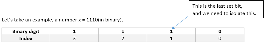
x&(-x) gives the last set bit in a number x. How? We use two's complement to represent negative numbers, write out the number in binary, then invert the digits, and add one to the result.
Example: x = 10(in decimal) = 1010(in binary)
Two's complement: 1010 -> 0101 + 1 = 0110
The last set bit is given by x&(-x) = (10)1(0) & (01)1(0) = 0010 = 2(in decimal)
Basic Idea of Binary Indexed Tree, We know the fact that each integer can be represented as sum of powers of two. Similarly, for a given array of size N, we can maintain an array BIT[] such that, at any index we can store sum of some numbers of the given array. This can also be called a partial sum tree.
Let’s use an example to understand how BIT[] stores partial sums.
//for ease, we make sure our given array is 1-based indexed
int a[] = {0, 1, 2, 3, 4, 5, 6, 7, 8, 9, 10, 11, 12, 13, 14, 15, 16};
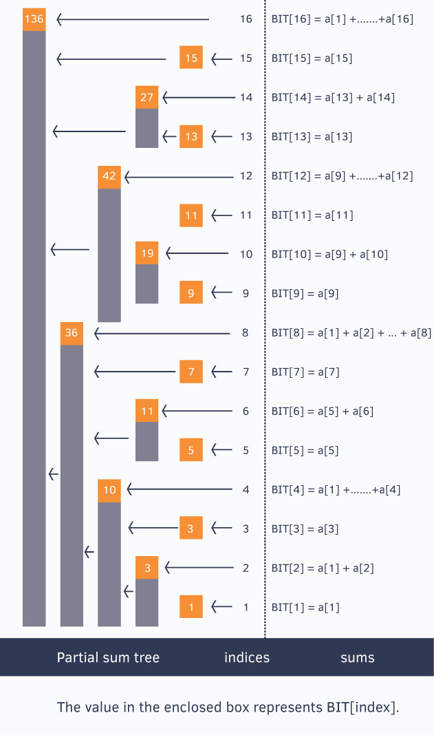
To generalize this every index i in the BIT[] array stores the cumulative sum from the index i to i - (1<<r) + 1 (both inclusive), where r represents the last set bit in the index i
Sum of first 12 numbers in array a[] = BIT[12] + BIT[8] = (a[12] + … + a[9]) + (a[8] + … + a[1])
Similarly, sum of first 6 elements = BIT[6] + BIT[4] = (a[6] + a[5]) + (a[4] + … + a[1])
Sum of first 8 elements = BIT[8] = a[8] + … + a[1]
Here’s the full program to solve efficiently
int BIT[1000], a[1000], n;
void update(int x, int delta)
{
      for(; x <= n; x += x&-x)
        BIT[x] += delta;
}
int query(int x)
{
     int sum = 0;
     for(; x > 0; x -= x&-x)
        sum += BIT[x];
     return sum;
}

int main()
{
     scanf(“%d”, &n);
     int i;
     for(i = 1; i <= n; i++)
     {
           scanf(“%d”, &a[i]);
           update(i, a[i]);
     }
     printf(“sum of first 10 elements is %d\n”, query(10));
     printf(“sum of all elements in range [2, 7] is %d\n”, query(7) – query(2-1));
     return 0;
}The word trie is an infix of the word “retrieval” because the trie can find a single word in a dictionary with only a prefix of the word.
Tripple-Array Trie, For a transition from state s to t which takes character c as the input, the condition maintained in the tripple-array trie is:
$check[base[s] + c] = s$ $next[base[s] + c] = t$
Double-Array Trie, For a transition from state s to t which takes character c as the input, the condition maintained in the double-array trie is:
$check[base[s] + c] = s$ $base[s] + c = t$
- Data Structures
- Using Tries
- An Implementation of Double-Array Trie
- Binary Trees
- Binary Indexed Trees
- Binary Indexed Tree or Fenwick Tree From Geeksforgeeks
- Binary Indexed Tree or Fenwick Tree From Hackerearth
- Preliminary Concepts: Negative Binary Numbers
- Two's Complement
- An Introduction to Binary Search and Red-Black Trees
- RedBlack Tree Visualization
- Red-black trees in 4 minutes
When comparing various sorting algorithms, there are several things to consider. The first is usually runtime. A second consideration is memory space. A third consideration is stability. Stability, simply defined, is what happens to elements that are comparatively the same. In a stable sort, those elements whose comparison key is the same will remain in the same relative order after sorting as they were before sorting. In an unstable sort, no guarantee is made as to the relative output order of those elements whose sort key is the same.
Bubble Sort, The idea is to pass through the data from one end to the other, and swap two adjacent elements whenever the first is greater than the last. This is O(n^2) runtime, and hence is very slow for large data sets.
for (int i = 0; i < data.Length; i++)
   for (int j = 0; j < data.Length - 1; j++)
      if (data[j] > data[j + 1])
      {
         tmp = data[j];
         data[j] = data[j + 1];
         data[j + 1] = tmp;
      }
Insertion Sort, an algorithm that seeks to sort a list one element at a time. One of the principal advantages of the insertion sort is that it works very efficiently for lists that are nearly sorted initially. Furthermore, it can also work on data sets that are constantly being added to.
for (int i = 0; i <= data.Length; i++) {
   int j = i;
   while (j > 0 && data[i] < data[j - 1])
      j--;
   int tmp = data[i];
   for (int k = i; k > j; k--)
      data[k] = data[k - 1];
   data[j] = tmp;
}
Merge Sort, A merge sort works recursively. First it divides a data set in half, and sorts each half separately. Next, the first elements from each of the two lists are compared. The lesser element is then removed from its list and added to the final result list. The runtime of this algorithm is O(n * log n)
int[] mergeSort (int[] data) {
   if (data.Length == 1)
      return data;
   int middle = data.Length / 2;
   int[] left = mergeSort(subArray(data, 0, middle - 1));
   int[] right = mergeSort(subArray(data, middle, data.Length - 1));
   int[] result = new int[data.Length];
   int dPtr = 0;
   int lPtr = 0;
   int rPtr = 0;
   while (dPtr < data.Length) {
      if (lPtr == left.Length) {
         result[dPtr] = right[rPtr];
         rPtr++;
      } else if (rPtr == right.Length) {
         result[dPtr] = left[lPtr];
         lPtr++;
      } else if (left[lPtr] < right[rPtr]) {
         result[dPtr] = left[lPtr];
         lPtr++;
      } else {
         result[dPtr] = right[rPtr];
         rPtr++;
      }
      dPtr++;
   }
   return result;
}
Heap Sort, we create a heap data structure. A heap is a data structure that stores data in a tree such that the smallest (or largest) element is always the root node. The runtime of a heap sort has an upper bound of O(n * log n).
Heap h = new Heap();
for (int i = 0; i < data.Length; i++)
   h.Add(data[i]);
int[] result = new int[data.Length];
for (int i = 0; i < data.Length; i++)
   data[i] = h.RemoveLowest();
Quick Sort, First, divide the data into two groups of “high” values and “low” values. Then, recursively process the two halves. Finally, reassemble the now sorted list. In a best case, the runtime is O(n * log n). In the worst case-where one of the two groups always has only a single element-the runtime drops to O(n^2).
Array quickSort(Array data) {
   if (Array.Length <= 1)
      return;
   middle = Array[Array.Length / 2];
   Array left = new Array();
   Array right = new Array();
   for (int i = 0; i < Array.Length; i++)
      if (i != Array.Length / 2) {
         if (Array[i] <= middle)
            left.Add(Array[i]);
         else
            right.Add(Array[i]);
      }
   return concatenate(quickSort(left), middle, quickSort(right));
}
Radix Sort, The radix sort was designed originally to sort data without having to directly compare elements to each other. A radix sort first takes the least-significant digit (or several digits, or bits), and places the values into buckets. If we took 4 bits at a time, we would need 16 buckets. We then put the list back together, and have a resulting list that is sorted by the least significant radix. We then do the same process, this time using the second-least significant radix. We lather, rinse, and repeat, until we get to the most significant radix, at which point the final result is a properly sorted list.
For example, let’s look at a list of numbers and do a radix sort using a 1-bit radix. Notice that it takes us 4 steps to get our final result, and that on each step we setup exactly two buckets:
{6, 9, 1, 4, 15, 12, 5, 6, 7, 11}
{6, 4, 12, 6} {9, 1, 15, 5, 7, 11}
{4, 12, 9, 1, 5} {6, 6, 15, 7, 11}
{9, 1, 11} {4, 12, 5, 6, 6, 15, 7}
{1, 4, 5, 6, 6, 7} {9, 11, 12, 15}
Radix sort visualization https://www.cs.usfca.edu/~galles/visualization/RadixSort.html
Binary search is used to quickly find a value in a sorted sequence (consider a sequence an ordinary array for now).
binary_search(A, target):
   lo = 1, hi = size(A)
   while lo <= hi:
      mid = lo + (hi-lo)/2
      if A[mid] == target:
         return mid
      else if A[mid] < target:
         lo = mid+1
      else:
         hi = mid-1

   // target was not found
a number of workers need to examine a number of filing cabinets. The cabinets are not all of the same size and we are told for each cabinet how many folders it contains. We are asked to find an assignment such that each worker gets a sequential series of cabinets to go through and that it minimizes the maximum amount of folders that a worker would have to look through.
10 20 30 40 50 60 70 80 90
10 20 30 40 50 | 60 70 | 80 90
the answer is 170 = 80 + 90 > 60 + 70 > 10 + 20 + 30 + 40 + 50
Solution: the minimum of the maximum amount of folders is SUM(all folders) / NUM(worker), so just binary search between SUM(all folders) / NUM(worker) and SUM(all folders).
The fundamental string searching (matching) problem is defined as follows: given two strings – a text and a pattern, determine whether the pattern appears in the text. The problem is also known as “the needle in a haystack problem.”
The “Naive” Method brute force, in the worst case it may take as much as (n * m) iterations to complete the task.
function NaiveSearch(string s[1..n], string pattern[1..m])
    for i from 1 to n-m+1
        for j from 1 to m
            if s[i+j-1] != pattern[j]
                jump to next iteration of outer loop
        return i
    return not found
Rabin-Karp Algorithm (RK), seeks to speed up the testing of equality of the pattern to the substrings in the text by using a hash function.
function RabinKarp(string s[1..n], string pattern[1..m])
    hpattern := hash(pattern[1..m]);
    for i from 1 to n-m+1
        hs := hash(s[i..i+m-1])
        if hs = hpattern
            if s[i..i+m-1] = pattern[1..m]
                return i
    return not found
The key to the Rabin–Karp algorithm's performance is the efficient computation of hash values of the successive substrings of the text. The Rabin fingerprint is a popular and effective rolling hash function. The Rabin fingerprint treats every substring as a number in some base, the base being usually a large prime. For example, 101.
hash("abr") = (97 × 101^2) + (98 × 101^1) + (114 × 101^0) = 999,509 rolling hash hash("bra") = [101^1 × (999,509 - (97 × 101^2))] + (97 × 101^0) = 1,011,309
Knuth–Morris–Pratt Algorithm
To illustrate the algorithm's details, consider a (relatively artificial) run of the algorithm, where W = "ABCDABD" and S = "ABC ABCDAB ABCDABCDABDE". At any given time, the algorithm is in a state determined by two integers:
- m, denoting the position within S where the prospective match for W begins,
- i, denoting the index of the currently considered character in W.
In each step the algorithm compares S[m+i] with W[i] and increments i if they are equal. This is depicted, at the start of the run, like
m: 01234567890123456789012
S: ABC ABCDAB ABCDABCDABDE
W: ABCDABD
i: 0123456
The algorithm compares successive characters of W to "parallel" characters of S, moving from one to the next by incrementing i if they match. However, in the fourth step S[3] = [ ] does not match W[3] = [D]. Rather than beginning to search again at S[1], we note that no 'A' occurs between positions 1 and 2 in W; hence, having checked all those characters previously (and knowing they matched the corresponding characters in S), there is no chance of finding the beginning of a match. Therefore, the algorithm sets m = 3 and i = 0.
m: 01234567890123456789012
S: ABC ABCDAB ABCDABCDABDE
W:    ABCDABD
i:    0123456
This match fails at the initial character, so the algorithm sets m = 4 and i = 0
m: 01234567890123456789012
S: ABC ABCDAB ABCDABCDABDE
W:     ABCDABD
i:     0123456
Here i increments through a nearly complete match "ABCDAB" until i = 6 giving a mismatch at W[6] and S[10]. However, just prior to the end of the current partial match, there was that substring "AB" that could be the beginning of a new match, so the algorithm must take this into consideration. As these characters match the two characters prior to the current position, those characters need not be checked again; the algorithm sets m = 8 (the start of the initial prefix) and i = 2 (signaling the first two characters match) and continues matching. Thus the algorithm not only omits previously matched characters of S (the "AB"), but also previously matched characters of W (the prefix "AB").
m: 01234567890123456789012
S: ABC ABCDAB ABCDABCDABDE
W:         ABCDABD
i:         0123456
This search at the new position fails immediately because W[2] (a 'C') does not match S[10] (a ' '). As in the first trial, the mismatch causes the algorithm to return to the beginning of W and begins searching at the mismatched character position of S: m = 10, reset i = 0.
m: 01234567890123456789012
S: ABC ABCDAB ABCDABCDABDE
W:           ABCDABD
i:           0123456
The match at m=10 fails immediately, so the algorithm next tries m = 11 and i = 0.
m: 01234567890123456789012
S: ABC ABCDAB ABCDABCDABDE
W:            ABCDABD
i:            0123456
Once again, the algorithm matches "ABCDAB", but the next character, 'C', does not match the final character 'D' of the word W. Reasoning as before, the algorithm sets m = 15, to start at the two-character string "AB" leading up to the current position, set i = 2, and continue matching from the current position.
m: 01234567890123456789012
S: ABC ABCDAB ABCDABCDABDE
W:                ABCDABD
i:                0123456
This time the match is complete, and the first character of the match is S[15].
A greedy algorithm, as the name suggests, always makes the choice that seems to be the best at that moment. This means that it makes a locally-optimal choice in the hope that this choice will lead to a globally-optimal solution.
- It is quite easy to come up with a greedy algorithm (or even multiple greedy algorithms) for a problem.
- Analyzing the run time for greedy algorithms will generally be much easier than for other techniques (like Divide and conquer). For the Divide and conquer technique, it is not clear whether the technique is fast or slow. This is because at each level of recursion the size of gets smaller and the number of sub-problems increases.
- The difficult part is that for greedy algorithms you have to work much harder to understand correctness issues. Even with the correct algorithm, it is hard to prove why it is correct. Proving that a greedy algorithm is correct is more of an art than a science. It involves a lot of creativity.
You are given an array A of integers, where each element indicates the time a thing takes for completion. You want to calculate the maximum number of things that you can do in the limited time that you have.
This is a simple Greedy-algorithm problem. In each iteration, you have to greedily select the things which will take the minimum amount of time to complete while maintaining two variables currentTime and numberOfThings.
A DP is an algorithmic technique which is usually based on a recurrent formula and one (or some) starting states. A sub-solution of the problem is constructed from previously found ones. DP solutions have a polynomial complexity which assures a much faster running time than other techniques like backtracking, brute-force etc.
Given a list of N coins, their values (v1, v2, … , vn), and the total sum s. Find the minimum number of coins the sum of which is s (we can use as many coins of one type as we want), or report that it’s not possible to select coins in such a way that they sum up to s.
Solution:
# dp[i] means the minimum number of coins the sum of which is i

dp = [-1] * s
for i in xrange(s):
    for j in xrange(n):
        if i < v[j]:
            continue
        if dp[i] == -1 or dp[i] > dp[i - v[j]] + 1:
            dp[i] = dp[i - v[j]] + 1
Given a sequence of N numbers – A1 , A2 , …, AN . Find the length of the longest non-decreasing sequence.
Solution:
# dp[i] means the length of the longest non-decreasing sequence up to Ai

dp = [1] * n
for i in xrange(n):
    for j in xrange(i):
        if a[i] >= a[j] and dp[j] + 1 > dp[i]:
            dp[i] = dp[j] + 1
The time complexity of above solution is O(N^2), the best solution is O(NLogN), check out further reading.
A table composed of N x M cells, each having a certain quantity of apples, is given. You start from the upper-left corner. At each step you can go down or right one cell. Find the maximum number of apples you can collect.
Solution:
# dp[i][j] means the maximum number of apples you can collect from upper-left corner to i * j cell.

dp = [[0] * m] * n
dp[0][0] = apple[0][0]
for i in xrange(n):
    for j in xrange(m):
        if i > 0 and dp[i][j] < dp[i - 1][j] + apple[i][j]:
            dp[i][j] = dp[i - 1][j] + apple[i][j]
        if j > 0 and dp[i][j] < dp[i][j - 1] + apple[i][j]:
            dp[i][j] = dp[i][j - 1] + apple[i][j]
Given an undirected graph G having positive weights and N vertices. You start with having a sum of M money. For passing through a vertex i, you must pay S[i] money. If you don’t have enough money – you can’t pass through that vertex. Find the shortest path from vertex 1 to vertex N
Solution:
# dp[i][j] means the length of the shortest path from vertex 1 to vertex i with j money left

dp[i][j - s[i]] = argmin(dp[k][j] + 1, if connected(k, i) and j - s[i] > 0)
Given a matrix with M rows and N columns (N x M). In each cell there’s a number of apples. You start from the upper-left corner of the matrix. You can go down or right one cell. You need to arrive to the bottom-right corner. Then you need to go back to the upper-left cell by going each step one cell left or up. Having arrived at this upper-left cell, you need to go again back to the bottom-right cell. Find the maximum number of apples you can collect. When you pass through a cell – you collect all the apples left there.
Solution:
# dp[i][j][k][l] means the maximum number of apples you can collect from the upper-left corner to row l at i, j and k col. a[i][j] means the number of apple.

dp[i][j][k][l] = max(
    dp[i][j][k][l-1] + a[i][l] + a[j][l] + a[k][l],
    dp[i - 1][j][k][l] + a[i][l],
    dp[i][j - 1][k][l] + a[j][l],
    dp[i][j][k - 1][l] + a[k][l])
Knapsack problem, Given a set of items, each with a weight and a value, determine the number of each item to include in a collection so that the total weight is less than or equal to a given limit and the total value is as large as possible.
Solution #1:
-
$m[0]=0$ (the sum of zero items, i.e., the summation of the empty set) - $m[w]=\max {w{i}\leq w}(v_{i}+m[w-w_{i}])$, where
$v_{i}$ is the value of the i-th kind of item.
Solution #2: Define
$m[0,,w]=0$ -
$m[i,,w]=m[i-1,,w]$ $if w_{i}>w$ , (the new item is more than the current weight limit) -
$m[i,,w]=\max(m[i-1,,w],,m[i-1,w-w_{i}]+v_{i})$ $ if w_{i}\leqslant w.$
- Dynamic Programming – From Novice to Advanced
- Longest Increasing Subsequence Size (N log N)
- Knapsack problem
For this popular algorithm interview question, the input will be a string consisting only of the characters 0, 1 and ?, where the ? acts as a wildcard that can be either a 0 or 1, and your goal is to print all possible combinations of the string. For example, if the string is "011?0" then your program should output a set of all strings, which are: ["01100", "01110"].