First steps
The following tutorial will guide you through your first steps with QuPath, and introduce you to the main features, buttons and concepts you need to get started. You will see how to:
- Open a whole slide image
- View image properties
- Navigate around images
- Manually annotate regions
- Detect cells
- View measurements
- Export results
- Save & reload your data
- Find help if you get stuck
Sidenotes like this are included to give extra information, or address something you might have noticed. You can safely ignore them if they don't seem relevant, or don't answer a question you actually had.
(My advice: read the sidenotes quickly as you go through in case they help immediately, but don't get too distracted by them. Then return to the tutorial after you've spent some more time using QuPath to check if they have any extra insights you can use.)
You can open an image with File → Open....
But that quickly becomes tiresome. A better plan is to simply drag the file you want to open onto QuPath's main window, and let QuPath do the rest. This also works for lots of other file types that QuPath can handle - not only images.
If you do not have a whole slide image handy, there are freely-available examples from the people at OpenSlide. Not all formats are fully-supported, but the Aperio folder is a good place to start. The H&E image used here is CMU-1.svs.
The Bio-Formats extension enables additional file formats.
The File → Open URL... option is only useful if any extra QuPath extensions are available for loading images hosted remotely. Currently, no such extensions are publicly available... but that will hopefully change.
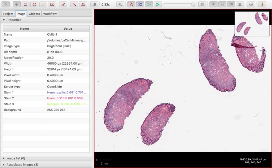
Usually, there's a panel on the left of the QuPath window: the Analysis panel. If not, click the Analysis panel button on the toolbar to open it ![]() .
.
There are a few tabs here that you will meet later. For now, click the Image tab to get a table of properties related to your image.
Most of these are fixed, but if you double-click on the right column of Image type you can adjust this if you like.
The image type might already be 'magically' set, because QuPath can make a guess when the image is open. This feature can be turned off under the Preferences
if you don't approve, or you find QuPath often gets it wrong.
To zoom in and out of an image within QuPath, use the scroll wheel of your mouse (or equivalent scrolling motion on a trackpad).
You can also jump to a specific magnification if you:
- Right-click on the image, and choose one of the zoom options e.g. Display → 100%, or
- Double-click on the little magnification box on the toolbar, and enter a value there.
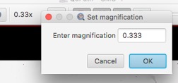
Double-clicking on the magnification box on the toolbar (here, the bit that shows 0.33x) opens an input dialog to enter a specific magnification.
To pan around a large image within QuPath, first make sure that the Move tool ![]() is selected in the toolbar. Then click anywhere on the image, and drag the mouse with the button held down to move.
is selected in the toolbar. Then click anywhere on the image, and drag the mouse with the button held down to move.
To move quickly, you can swipe more vigorously and release the button at the end to 'fling' the image elsewhere.
Alternatively, you can click on the Overview image in the top right to automatically jump to a specific region.
For other methods to navigate large images - including multitouch support for touchpads, touch-sensitive screens and 3D mice - see Viewing images.
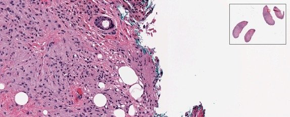
Clicking on the image overview (top right) shifts to view another part of the image.
Understanding objects is key to making sense of QuPath's features.
You can think of an object informally as something in an image that QuPath can identify, classify and measure.
For now, we only care about two kinds of objects:
- Annotations: Objects that you usually create yourself, by drawing on the image
- Detections: Objects that QuPath usually creates for you, e.g. by detecting cells (where each cell is an object)
Usually, you end up with a small number of annotations relating to larger regions (e.g. entire areas of tissue). But you can have potentially millions of detections. So for this reason QuPath handles and displays them a bit differently - but they also share a lot of similarities, in that you can see them both drawn on top of images and measure.
For a purely manual analysis - drawing regions on an image and measuring them - you may find that you don't need detections at all... annotations are enough.
If you've used ImageJ, objects perform much of the same function as ImageJ's ROIs (Regions of interest). However objects are a bit more sophisticated: they not only represent regions, but they also have their own lists of measurements and classifications, and can store relationships to other objects as well. This distinction is part of what makes QuPath a better fit for some applications (such as digital pathology), while ImageJ may be preferable for others.
For a deeper discussion of objects and why they matter so much, see the QuPath concepts section.
Create your first annotation object by drawing a rectangle on top of the image. Do this by clicking on the Rectangle tool ![]() to select it, then click and drag over a region in the image. When releasing the mouse button, the rectangle should remain drawn on top of the image.
to select it, then click and drag over a region in the image. When releasing the mouse button, the rectangle should remain drawn on top of the image.
Now try drawing several more annotations of different shapes around different areas in the image using the Ellipse ![]() , Polygon
, Polygon ![]() and Brush tools
and Brush tools ![]() .
.
Most of QuPath's drawing tools work similarly (i.e. select the tool, click on the image, drag the mouse), but note that the polygon tool also allows you to eschew dragging and instead click each point where you want a vertex on the polygon. Double-click to set the final point.
By default, QuPath will switch back to the Move tool
after you've drawn an annotation with any tool except the Brush. This is to help accidentally drawing new annotations when you really just wanted to move around in the image or do something with an existing annotation. The Brush is different, because it's commonly used to paint or edit multiple regions at a time, and it can be annoying to have to switch it back on regularly.
If you don't like the default behavior, it can be changed with the Return to Move Tool automatically option in the Preferences
Either way, you can quickly activate the tool you want using a shortcut key, e.g. just type M for Move, B for Brush, P for Polygon etc. You can see all the shortcut keys for drawing tools under the Tools menu.
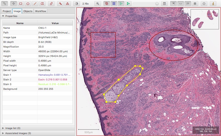
You should find that when you draw an annotation object, it is initially selected. In the screenshot above, the selected (polygon) annotation is shown in yellow - with little square handles indicating vertices that could be adjusted if necessary.
Usually, you want to make sure an object is selected before you can do something with it. If the object you want isn't selected already, return to the Move tool ![]() , either by clicking on the tool button or pressing M, and then double-clicking on it to select it.
, either by clicking on the tool button or pressing M, and then double-clicking on it to select it.
By default, selections are shown in yellow. You can change this color in the Preferences
If you like, you can select multiple annotations by clicking on them while holding down the Alt key.
Return now to the Analysis panel (left of the screen, ![]() ) and click on the Annotations tab.
) and click on the Annotations tab.
Note: in earlier QuPath versions, the tab to select was called Objects... which is why the screenshot is different.
You should see a list of your annotations here. Clicking on this list gives another way to select an object. But you can also set the properties of your annotations here if you like. One way is to select from a predefined list of classifications on the right, and choose Set class. Alternatively, right-click on any listed annotation and choose Set properties to choose any arbitrary name or color.
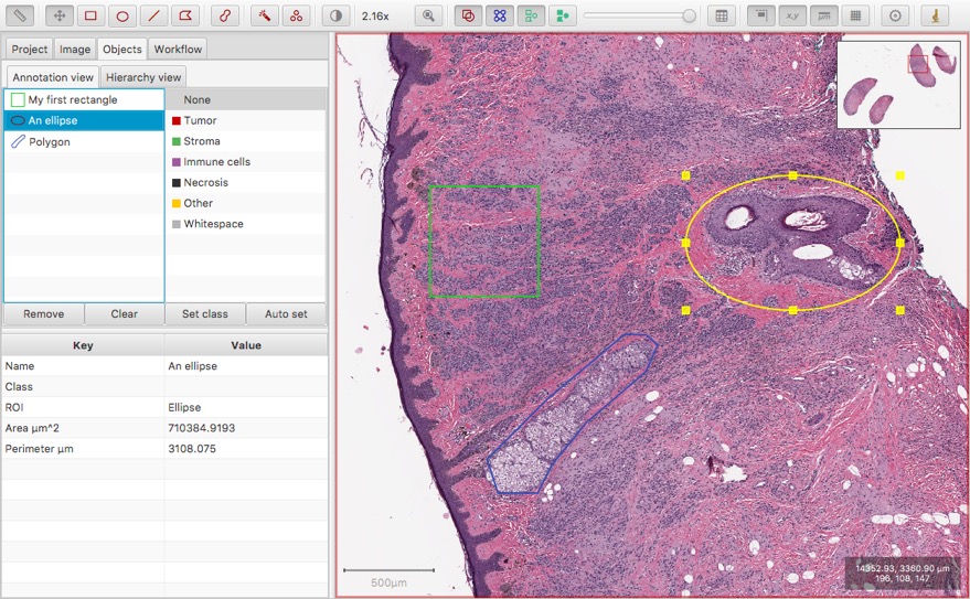
Still in the Analysis panel, below the annotation list you should see a table showing measurements for the currently-selected object. This should update automatically if you click on another annotation.
If you draw an annotation you don't like, you can delete it from the annotation list. Alternatively, if you're currently working inside the viewer (moving around, drawing annotations) you can simply press the backspace or delete key to remove the currently-selected objects.
Mostly, this 'just works'. But if you are deleting an object that contains other objects inside it, then QuPath will ask you if you want to 'Keep the descendant object(s)'. If you click Yes (or press Enter), this only the selected object will be removed. If you click No, then both the selected annotation and all the annotations inside it will be removed. If you click Cancel, nothing will be removed.
For more information on the strange use of the word descendant, see Object hierarchies.
Next, try creating detection objects inside an annotation. First, draw an annotation in an area of the image containing cells - ideally quite small, to contain perhaps 100 cells.
Run the Analyze → Cell analysis → Cell detection command. This should bring up an intimidating list of parameters to adapt the detection to different images. If you like you can explore these, and hover the mouse over each parameter for a description - but for now, you can also just ignore them and use the defaults (which tend to behave sensibly across a range of images).
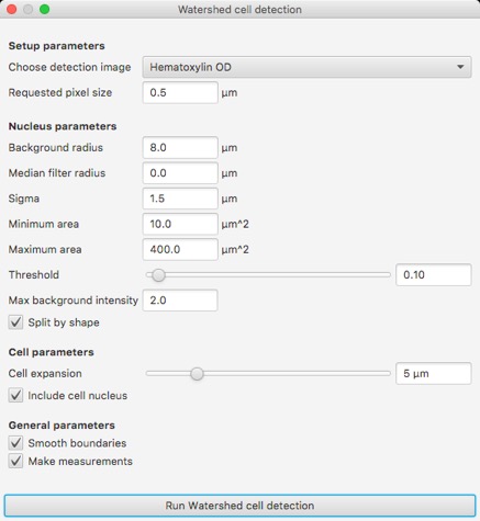
Press the Run button at the bottom of the dialog. After a few seconds, cells should appear in the area you have selected.
These cells are your first detection objects.
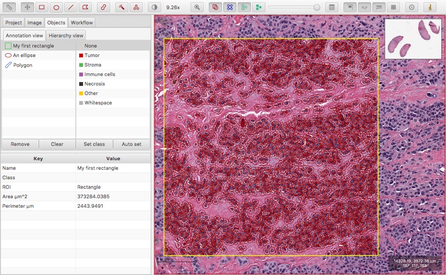
Detection objects also have measurements, like annotation objects. You can select them, and their measurements show up in the same table in the Analysis panel. But you should see that detection objects look a bit different on screen. For example, if you zoom out to a low magnification, you should see annotations are still clearly visible, drawn with thick lines. However detections get smaller, their outlines get thinner, and they start to merge into one another.
This is because annotations and detections serve different purposes. Detections relate to small structures, such as cells or nuclei, of which you can easily end up with hundreds of thousands - or even millions - within a single image. You need to zoom in to see them. However you will generally have a much smaller number of annotations - each related to quite a large area - and you need to be able to see them when zoomed out.
The pattern we applied here here is common in QuPath:
- Create an annotation (usually by drawing it)
- Run a command to get QuPath to detect objects inside the annotation
In case this seems horribly manual, be assured that it's possible to get QuPath to detect across many annotations simultaneously - and even to create annotations automatically. Just not in Lesson #1.
As your collections of objects grow on the image, it may start to become cluttered or confusing. There are four useful toolbar buttons that can help customize how the objects are displayed. These are:
-
 Show and hide annotations - shortcut A
-
 Show and hide a TMA grid (only relevant for Tissue microarrays) - shortcut G
-
 Show and hide detections - shortcut H (for 'hide')
 -
 Fill and unfill detections - shortcut F
These allow you to quickly toggle on and off your markup to see switch between looking at analysis data and the underlying image.
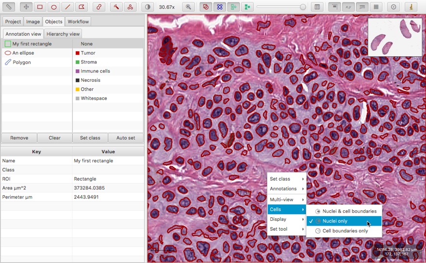
You can also right-click on the image, and further modify how cells are displayed, i.e. with/without nuclei or boundaries shown.
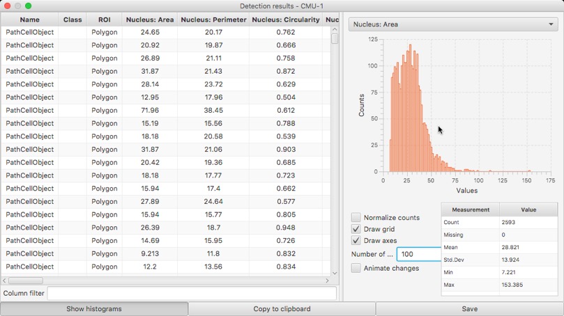
You can generate a results table containing measurements for your objects by selecting the Table button in the toolbar ![]() . You can then choose whether you want your table to contain annotations or detections.
. You can then choose whether you want your table to contain annotations or detections.
Note that this table remains connected to the image, and allows you to select individual objects, or sort by columns. You can also generate histograms for any measurements, and save the table to a CSV file or copy its contents for pasting into another application, e.g. Excel.
When you're done, you can save your analysis with File → Save As..., or by responding positively to any saving prompts whenever you try to open another image or to quit.
This will save a .qpdata file, which is QuPath's primary file format for storing objects and other image-related data. Note that this does not actually store the image itself (which may be huge), but rather only a link to it.
You can reopen .qpdata files in the same way as you could open any image - by dragging it onto the QuPath viewer, or by choosing File → Open.
It's not necessary to open your image again first. If your original image remains where it was, the link within the .qpdata file will be used to open it automatically. However if the image has been moved, QuPath will show a dialog prompting you to select the new image location.
If you got this far, great! You've seen many of the main features of QuPath, and had your first encounter with the fundamental idea of working with objects.
Even if not everything is clear yet, hopefully it gives enough motivation to read on through the documentation and see how powerful these ideas can become when put together.