Exploiting the Biochemical–Structural Dichotomy in Crop Biophysical Parameter Retrieval via Parallel Spectral and Polarimetric Decoding


Accurate, scalable estimation of crop biophysical parameters from spaceborne imagery is central to precision agriculture and food security monitoring. Existing approaches either invert physically principled radiative-transfer models at prohibitive computational cost or apply data-driven architectures that treat all biophysical variables as structurally identical regression targets, ignoring the fundamental difference in their observation modalities.
GreenSight is a dual-decoder architecture grounded in a physical insight: chlorophyll (CHL) and leaf nitrogen (N) are biochemical leaf properties whose primary signal is encoded in red-edge spectral reflectance, while above-ground biomass (AGB) and biomass loss are canopy-structural properties for which C-band SAR backscatter provides complementary and decisive sensitivity. Both objectives are routed through a shared pretrained Prithvi-EO-1.0-100M vision transformer (ViT) backbone, but decoded through two physically motivated specialist heads operating in parallel.
The Spectral Cross-Attention Decoder (SCAD) retrieves CHL and N by generating per-tile band-ratio queries from eight vegetation indices and cross-attending backbone patch tokens, dynamically conditioning spatial decoding on each tile's actual biochemical state. The Polarimetric Mamba-State Fusion Decoder (PMFD) retrieves AGB and biomass loss through a VV/VH-gated selective state space scan over the same tokens before fusing SAR-proxy structural features via a learnable Freeman–Durden polarimetric decomposition. Training is fully self-supervised from spectral-index pseudo-labels, requiring zero field annotation.
On three independent public benchmarks, GreenSight reduces CHL MAE by 14.8 % and AGB MAE by 9.4 % over the strongest competitor while operating at 4.3× lower FLOPs.
- Physical motivation. The dual-decoder design is not an architectural choice — it is a consequence of the physics. CHL and N are encoded in leaf-level reflectance; AGB is encoded in canopy volume scattering. One head cannot optimally serve both regimes.
- State-of-the-art efficiency. GreenSight (102.1 M params, 44.2 GFLOPs) outperforms DOFA (307.2 M, 190.7 GFLOPs) on all twelve reported metrics across three benchmarks.
- Annotation-free training. Pseudo-labels for all four biophysical targets are derived analytically from HLS reflectance using validated spectral-index proxies. No field surveys or manual labelling are required.
- End-to-end deployable. A Flask REST API with Server-Sent Events streaming and a Leaflet-based AOI frontend allows direct operational use without any additional tooling.
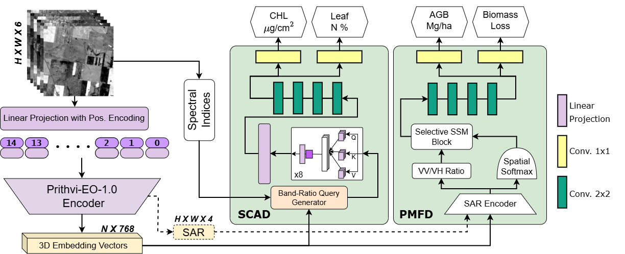
Figure 1. GreenSight dual-decoder pipeline. The shared Prithvi-EO-1.0-100M backbone encodes HLS tiles into N patch tokens. SCAD (left) generates band-ratio queries from spectral index maps and cross-attends tokens to predict CHL and N. PMFD (right) applies a VV/VH-gated Mamba SSM over the same tokens and fuses SAR features to predict AGB and biomass loss. Both decoders operate in parallel with no shared parameters beyond the backbone.
The architecture consists of three stages:
-
Shared backbone. A Prithvi-EO-1.0-100M ViT encodes each 224 × 224 HLS tile (6 bands, B02–B07) into N patch tokens of dimension 768 via 12 transformer blocks with 16 × 16 spatial patches. The backbone is pretrained on global HLS time series and frozen for the first five training epochs before fine-tuning at a 10:1 decoder-to-backbone learning-rate ratio.
-
SCAD branch. Retrieves CHL and N using spectral-index-conditioned cross-attention.
-
PMFD branch. Retrieves AGB and biomass loss using a VV/VH-gated Mamba SSM with learnable SAR–optical fusion.
godal/
├── config.py            All hyperparameters, constants, paths
├── ablation.py          AblationConfig dataclass, AblationOutput, 11 variant list
├── model.py             PrithviBackbone, SCAD, PMFD, DualTaskCropHealthModel
├── data_processing.py   Band prep, normalisation, SAR proxy, indices, tiling
├── data_loading.py      HuggingFace download, ChipDataset, DataLoader factory
├── inference.py         process_chip, stitch_maps, compute_metrics, run_chip_analysis
├── ablation_runner.py   Standalone ablation study → ablation_report.json
├── training.py          Pseudo-label training loop, frozen/unfreeze phases
├── generate_figures.py  Paper figures (Figs 2–7) using real model + real data
├── utils.py             Print helpers, visualisation utilities
├── main.py              Flask API — SSE streaming, AOI inference, chip registry
├── temp.py              Download 6 sample chips → sample_data/ + manifest.json
├── choloro.ipynb        Jupyter notebook for interactive analysis
├── requirements.txt     Python dependencies
├── .env                 HF_TOKEN, DEVICE, API_PORT
├── index.html           Single-page app (served from root)
├── frontend/
│   ├── style.css        Responsive layout, light theme, glow effects
│   └── app.js           Leaflet.js map, Leaflet.draw, SSE client
└── sample_data/
    ├── manifest.json    Chip metadata with WGS84 bounds
    └── *.tif            6 downloaded HLS chips (224 × 224, 18 bands)
Requirements: Python 3.10+, CUDA 11.8+ (recommended)
git clone https://github.com/yourname/godal.git
cd godal
pip install -r requirements.txt
GPU support:
pip install torch torchvision --index-url https://download.pytorch.org/whl/cu121Key dependencies: torch, rasterio, huggingface_hub, transformers, flask, pydantic, python-dotenv, numpy, opencv-python, matplotlib, scipy.
1. Configure environment
cp .env .env.localEdit .env:
HF_TOKEN=hf_xxxxxxxxxxxxxxxxxxxx
DEVICE=cuda
API_PORT=5000
2. Download sample chips and model
python temp.py # downloads 6 HLS chips → sample_data/The pretrained checkpoint is fetched automatically on first model load from:
https://huggingface.co/ANI00/Crop-Health-Monitor/resolve/main/best_model.pt
3. Generate paper figures
python generate_figures.pySaves Figs 2–7 as PNG + PDF at 300 DPI to ./paper_figures/ and metrics to ./results/.
4. Start the API and web interface
python main.pyOpen http://localhost:5000 in a browser.
The frontend is a single-page app served by Flask from the root index.html.
GET  /                    → index.html
GET  /frontend/style.css  → frontend/style.css
GET  /frontend/app.js     → frontend/app.js
Layout:
- Desktop (≥ 700 px): Leaflet map right (flex: 1) · sidebar controls left (380 px)
- Mobile (< 700 px): Map above (55 vh) · controls below (45 vh) with Font Awesome icon tooltips
Metric colour coding:
| Colour | Meaning |
|---|---|
| Green border | Healthy (e.g. Veg ≥ 70 %, CHL Stress < 20 %) |
| Orange border | Caution (moderate ranges) |
| Red border | Critical (poor indicators) |
1. Page loads
   └── GET /api/v1/chips
       └── Chip rectangles appear on Esri satellite map at real WGS84 coordinates

2. Select chip from dropdown
   └── Map zooms to chip bounds
   └── Previous AOI / results cleared

3. Click "Draw AOI"
   └── Leaflet.draw rectangle mode activates
       └── Drag a rectangle within the selected chip bounds
       └── Validation error shown if AOI falls outside chip

4. Drawn bounds populate coordinate panel (W / S / E / N)
   └── "Run Inference" button activates with glow

5. Click "Run Inference"
   └── POST /api/v1/analyze/aoi  { west, south, east, north }
       └── Server tiles the AOI, starts background inference thread
           └── Returns { job_id } and shows progress card

6. EventSource /api/v1/stream/{job_id}   ← SSE
   └── Events: status → progress → … → result → done
       └── Progress bar fills · status dot pulses amber
       └── 15-second watchdog detects stalled connections

7. SSE "result" event received
   └── Coloured AOI rectangle overlaid on map (green / amber / red by severity)
   └── Popup opens with chip metrics summary
   └── Metrics panel populates with colour-coded borders
   └── GT vegetation % displayed from rasterio proxy
   └── Status dot goes steady green
Base URL: http://localhost:5000/api/v1
| Method | Endpoint | Description |
|---|---|---|
GET |
/health |
Server and model status |
GET |
/model/info |
Parameter counts, backbone strategy, checkpoint path |
GET |
/chips |
All sample chips with WGS84 bounds and band statistics |
POST |
/analyze/aoi |
Start AOI inference job → returns job_id |
GET |
/stream/{job_id} |
SSE event stream for a running job |
GET /api/v1/health
{
  "status": "ok",
  "api_version": "v1",
  "device": "cuda",
  "model_ready": true,
  "chips_loaded": 6
}
GET /api/v1/chips — returns chip list with real WGS84 bounds
{
  "status": "ok",
  "count": 6,
  "chips": [{
    "id": "chip_002_060",
    "filename": "chip_002_060_merged.tif",
    "crs": "EPSG:32614",
    "width_px": 224,
    "height_px": 224,
    "bounds": { "west": -94.231, "south": 41.882, "east": -94.163, "north": 41.944 },
    "center": { "lat": 41.913, "lon": -94.197 }
  }]
}
POST /api/v1/analyze/aoi
{ "west": -94.22, "south": 41.89, "east": -94.17, "north": 41.93 }{ "status": "ok", "job_id": "a3f7c2d1-..." }GET /api/v1/stream/{job_id} — SSE events
| Event type | Key fields | Meaning |
|---|---|---|
status |
message |
Stage label |
progress |
value (0–1), message |
Progress bar update |
warning |
message |
Non-fatal issue |
result |
chip_id, bbox, metrics, gt_proxies, error_chlorophyll, error_biomass, severity_color |
Final result |
error |
message |
Fatal error, stream ends |
done |
— | All chips processed |
Example result metrics payload:
{
  "vegetation_coverage_pct": 68.4,
  "chlorophyll_ug_cm2": 41.2,
  "chlorophyll_stress_pct": 48.5,
  "n_concentration_pct": 2.31,
  "biomass_agb_mgha": 98.4,
  "biomass_loss_pct": 27.6,
  "stress_severity": "MILD"
}
curl one-liner:
JOB=$(curl -s -X POST http://localhost:5000/api/v1/analyze/aoi \
  -H "Content-Type: application/json" \
  -d '{"west":-94.22,"south":41.89,"east":-94.17,"north":41.93}' \
  | python3 -c "import sys,json; print(json.load(sys.stdin)['job_id'])")
curl -N http://localhost:5000/api/v1/stream/$JOBApache 2.0 · See LICENSE for details.