Adaptive, occupation-certified spectral calculations on simplex meshes.
FermiSimplex finds Fermi surfaces and computes zero-temperature charge and density matrices without paying for a dense momentum grid. Its central object is the local occupation
and its central question is simple: can the occupation be proved constant on this simplex, or should we look more closely?
The upstream development repository is GitLab; the GitHub repository is a public mirror.
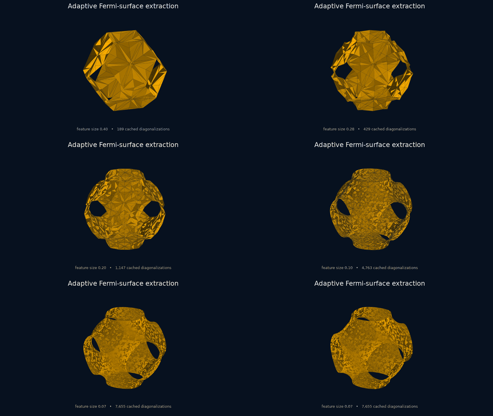
See the visual Python tour for a presentation-ready introduction with real adaptive sampling traces, multiband examples, and a rotating noble-metal-inspired three-dimensional surface.
- 🛡️ Gapped-region proofs combine cached eigensystems with rigorous spectral bounds to exclude a Fermi-level crossing throughout a simplex and to bound the remaining charge.
- ⚡ Adaptive sampling, built on AdaptiveSimplex, concentrates diagonalizations near unresolved Fermi surfaces instead of refining the entire Brillouin zone uniformly.
- 🚀 Numerical efficiency by design: adaptive refinement, shared spectral caching, and the compiled numerical core avoid repeated work as the Fermi surface becomes progressively sharper.
- 🎯 Projected charge estimates compare sampled projected eigenvalues with vertex-linear interpolation only in the bands whose occupation is still ambiguous.
- 🧩 Python and C++ share one numerical core; models can be dense callables or translation-invariant tight-binding Hamiltonians.
From a source checkout with a C++20 compiler and BLAS/LAPACK available:
pip install .The model below produces the three-dimensional surface shown above:
import numpy as np

from fermisimplex import SpectralMesh


def hamiltonian(kx, ky, kz):
    phase = 2 * np.pi * np.array([kx, ky, kz])
    return np.array([[np.cos(phase).sum()]], dtype=complex)


mesh = SpectralMesh(hamiltonian)
surface = mesh.fermi_surface(
    mu=0.17,
    min_feature_size=0.07,
    curvature_bound=(2 * np.pi) ** 2,
)

surface.points      # (npoints, 3)
surface.cells       # (ntriangles, 3)
surface.cell_bands  # band index for every triangle
The coordinates are reduced coordinates in SpectralMesh infers the momentum-space dimension from the
callable arguments and the matrix dimension by evaluating it at the origin.
Callables receive separate coordinates: hamiltonian(kx, ky, ...).
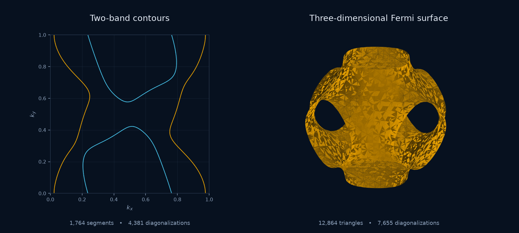
The same SpectralMesh can drive the other observables and reuse every
eigensystem it has already computed:
charge = mesh.integrate_charge(
    mu=0.17,
    target_error=1e-2,
    max_refinements=10_000,
    curvature_bound=(2 * np.pi) ** 2,
)
density = mesh.integrate_density_matrix(
    mu=0.17,
    lattice_vectors=[(0, 0, 0), (1, 0, 0)],
    target_error=1e-2,
    max_refinements=10_000,
)

charge.value
charge.stopping_error
charge.certified_error_bound
density.matrices  # (number of lattice vectors, ndof, ndof)
For a tight-binding model,
pass {R: H_R, ...} directly to SpectralMesh. Opposite hoppings are checked
for
At each simplex, FermiSimplex asks: can the occupation change between the
sampled vertices? It combines their eigensystems with curvature_bound,
which limits how much the Hamiltonian can bend in between. If occupied and
unoccupied trial subspaces remain on opposite sides of
- Certified: no Fermi surface crosses the simplex.
- Partially certified: rigorous lower and upper occupation bounds remain.
- Inconclusive: this is not a gapless verdict; FermiSimplex refines and tries again.
Every charge and Fermi-surface simplex is checked. The remaining uncertainty
becomes charge.certified_error_bound; surface.coverage_certified concerns
classification down to min_feature_size, not topology or geometric accuracy.
Density matrices currently use adaptive estimates instead.
The guarantee assumes a valid curvature_bound. Omitting it, None, and
0.0 all assert zero curvature; none disables certification. See the
mathematics guide for the proof and error bounds.
-
SpectralMesh: accept a callable or tight-binding dictionary and own the adaptive geometry and cached eigensystems. -
certify_simplex: certify supplied vertex eigenpairs directly; eigenvalues must be finite and ascending, and eigenvector columns must be finite and orthonormal. These performance-sensitive numerical preconditions are not rechecked. -
mesh.integrate_charge: adaptive filling and$dQ/d\mu$ . -
mesh.integrate_density_matrix: real-space density-matrix components. -
mesh.fermi_surface: band-labelled points and cells in reduced coordinates.
Adaptive controls such as target_error, max_refinements, and
preview_depth are ordinary keyword arguments on the calculation that uses
them—there is no separate options object. Charge calculations default to
preview_depth=0 because their sampled projected-error estimate drives
refinement intrinsically; positive depths are intended for explicit
diagnostic comparisons.
See the visual Python tour, runnable quick start, and two-band plotting example, the visual-generation notes, and the build and architecture guide.
AdaptiveSimplex provides the mesh geometry, refinement, vertex caching, and cut-simplex integration; FermiSimplex adds the spectral models, certificates, and observable-specific algorithms.
pixi run testThis builds the standalone C++ library, verifies an installed downstream CMake consumer, rebuilds the Python extension, and runs the Python tests. The dense 60-band stress case lives in benchmarks/fermi_surface_60.py.
FermiSimplex is licensed under the BSD 3-Clause license. If you use it in research, please cite the metadata in CITATION.cff.