ASWIFT

View ASWIFT on PyPI

ASWIFT fits square-wave voltammetry (SWV) traces and extracts peak signal, background, peak voltage, and full-prominence peak width. Use the no-code ASWIFT Viewer for interactive analysis, or install the Python package to build ASWIFT into a custom workflow.

Setup

ASWIFT is available as a standalone desktop application and as a Python package. The standalone application includes everything needed to run the viewer; Python is not required.

Install the desktop application

Precompiled applications are available from the ASWIFT 1.0.2 GitHub Release. Download the archive that matches your computer:

Download	System
ASWIFT-Viewer-macos-arm64.zip	Apple Silicon Mac (M1, M2, M3, M4, or newer)
ASWIFT-Viewer-macos-x64.zip	Intel-based Mac
ASWIFT-Viewer-windows-x64.zip	64-bit Windows

Unzip the archive, then open ASWIFT Viewer. Because ASWIFT is distributed outside the Apple App Store and Microsoft Store, your operating system may show a security warning the first time it opens. Follow the system prompt to allow the application to run; on macOS, this may require approval under Privacy & Security.

Install the Python package

ASWIFT requires Python 3.12 or newer. Install the core fitting utilities with:

pip install aswift

Install the viewer, pandas CSV helpers, plotting tools, and PalmSens .pssession support with:

pip install "aswift[viewer]"

PalmSens support uses pypalmsens, which requires the Microsoft .NET 9 Runtime. If ASWIFT reports that it could not create a .NET runtime or CoreCLR, install the runtime and restart ASWIFT.

Activate the Python environment in which ASWIFT was installed, then launch the viewer:

aswift-viewer

Example notebooks for SWV fitting, CSV workflows, and PalmSens data are in the examples directory.

Using the ASWIFT Viewer

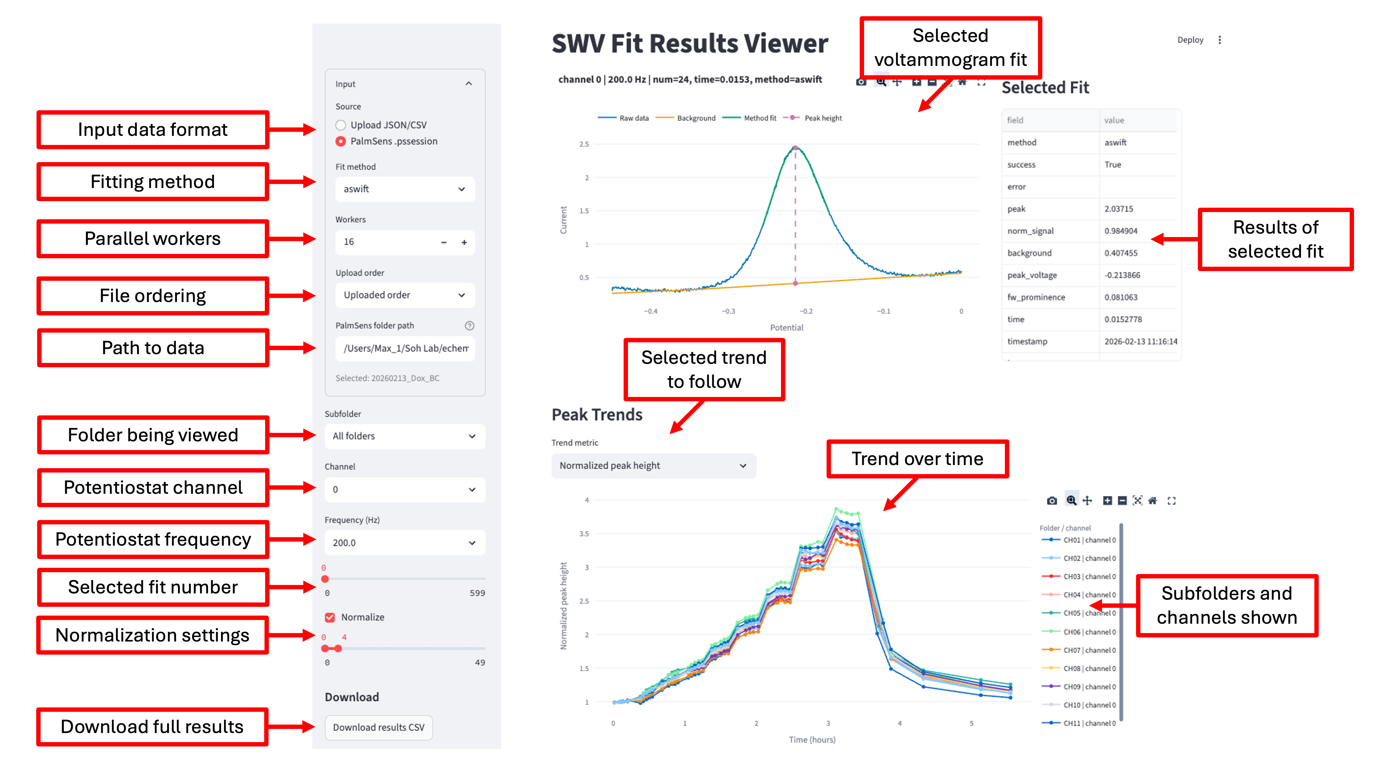
The viewer displays the selected voltammogram and its fitted background and peak, a table of values extracted from that fit, and a trend plot across the full dataset.

Load data

Choose an input source in the sidebar, then upload one or more SWV data files or enter the path to a directory containing a PalmSens dataset. Download correctly formatted sample files from the v1.0.2 example-data archive.

ASWIFT supports three input formats:

• PalmSens .pssession: Select PalmSens .pssession and enter a folder containing .pssession files. Subfolders are searched automatically. ASWIFT extracts available frequency, acquisition time, and channel metadata and saves processed results as a structured JSON file in the selected directory. While the viewer remains open, newly added files are detected and processed automatically. Files accidentally downloaded with a .pssession.mp3 suffix are renamed before processing.

• CSV: Upload either a simple sweep with voltage in the first column and one or more current traces in subsequent columns, or a structured table with one complete voltammogram per row plus metadata such as channel and frequency. Simple sweeps may have a header row or no header row. UTF-8, UTF-8 BOM, UTF-16, and Latin-1 encodings are accepted.

• JSON: Upload structured fit results previously generated by ASWIFT. This lets you reopen, visualize, and analyze a processed dataset without fitting the raw data again.

If a trace cannot be fit but its raw voltage and current are available, the viewer still displays the raw trace for inspection.

Inspect and process results

Use the sidebar controls to choose what appears in the fit and trend plots:

• Fit method: Choose the ASWIFT or polynomial-linear fitting method.
• Workers: Increase the number of worker processes to accelerate larger datasets on multi-core computers.
• Upload order: Keep uploaded order or sort uploaded files by file name.
• Subfolder: Choose which PalmSens subfolder to inspect, or show all folders together.
• Channel: Choose the potentiostat channel for the individual fit. Trend plots initially show all channels; click legend entries to hide or show them.
• Frequency: Choose the SWV frequency shown in the individual fit and trend plots.
• Sample index: Step through voltammograms for the selected folder, channel, and frequency. Samples are ordered by acquisition time when a timestamp is available and by upload order otherwise.
• Normalize: Normalize peak heights to the average over a selected reference range. Normalization is calculated independently for every subfolder, method, frequency, and channel.

The Trend metric menu switches the time or measurement series among peak height, peak voltage, and full-prominence peak width when those values are available. Use the plot legend and toolbar to explore individual series.

Select Download results CSV at the bottom of the sidebar to export raw and normalized results with their associated metadata.

Python API

Fit and plot one trace

import numpy as np
from aswift import aswift_fit, plot_fit_result, poly_linear_fit

volts = np.asarray([...], dtype=float)
current = np.asarray([...], dtype=float)

result = aswift_fit(volts, current)
# Alternative model:
# result = poly_linear_fit(volts, current)

print(result.peak_signal, result.peak_voltage)
ax = plot_fit_result(result)

The returned FitResult contains:

• peak_signal: background-subtracted peak height
• peak_background: background current at the peak
• peak_voltage: voltage at the peak maximum
• fw_prominence: full-prominence peak width
• peak_profile: fitted peak-only profile
• background_profile: fitted background profile
• fitted_current: combined peak and background profiles

Fit a structured dataframe

Use one row per voltammogram. The voltage and current columns each contain the full array for that trace; additional metadata columns such as file, hz, num, channel, and time are preserved. This workflow requires the batch, plot, or viewer extra.

from aswift import fit_dataframe, results_to_signal_table

results = fit_dataframe(df, method="aswift", n_workers=1)
signals = results_to_signal_table(
    results,
    calibration_lower_idx=0,
    calibration_upper_idx=4,
)

For large CPU-bound batches, independent traces can be fit in separate processes:

results = fit_dataframe(
    df,
    method="aswift",
    n_workers=4,
    parallel_backend="process",
    chunksize=16,
)

Single-worker fitting avoids process startup and serialization overhead and is often faster for small interactive datasets. Benchmark representative data before increasing n_workers.

Load PalmSens files

from aswift import fit_pssession_folder, pssession_folder_to_dataframe

df = pssession_folder_to_dataframe("path/to/pssession/folder", recursive=True)
df, results = fit_pssession_folder(
    "path/to/pssession/folder",
    recursive=True,
    n_workers=1,
)

ASWIFT orders traces using available timestamp, frequency, file number, and channel metadata. Elapsed time is reported in hours from the earliest measurement.

Development

Install the developer dependencies and run the test suite from the repository root:

python -m venv venv
source venv/bin/activate
python -m pip install -e ".[developer]"
NUMBA_CACHE_DIR=/private/tmp/numba-cache python -m pytest -q

Verify the distributable package with:

python -m build

Desktop packaging and release instructions are documented in release_assets/README.md. The maintainer checklist for publishing GitHub and PyPI releases is in docs/RELEASING.md.

Bug reports and feature requests

Please open a GitHub issue for bug reports, questions, feedback, or feature requests.

Citation

If you use ASWIFT in your research, please cite:

Yates, M., Ji, J., Yee, S., & Soh, H. T. (2026). Robust Regularization Enables Automated, Real-Time Square-Wave Voltammetry Signal Quantification. bioRxiv. https://doi.org/10.64898/2026.07.25.740173

Machine-readable citation metadata is available in CITATION.cff.

Acknowledgments

This work was supported by resources provided by the Soh Lab within Stanford University's School of Engineering. The authors thank Stan Yates for his development and consulting contributions in preparing ASWIFT for distribution as a PyPI package.

Author

Max Yates - PhD Candidate - GitHub profile

License

ASWIFT is licensed under the MIT License. See LICENSE for details.