Plotting

Plotting (fastCDS plot)

Once you have an isoform_structure.tsv from Mapping, fastCDS plot renders it as a static figure or as an interactive viewer. That TSV is the plotter's only input - it is written by --output isoform or the default --output all, so a plain fastCDS map produces it; the coding / introns / span / bed12 outputs are BED/TSV tracks for a genome browser, not plotter input. There is one output flag, --out, and its extension picks the format: .pdf / .png / .svg give a static matplotlib figure, and .html gives the interactive viewer. For .html, --engine chooses the renderer - a self-contained vanilla-JS viewer (js, the default, no dependencies) or plotly. The plotter reads the TSV directly and never re-derives coordinates from the genome, so anything you can express by editing the table is plottable.

Together with the BED12 track written by Mapping, these are fastCDS's three output types: the BED12 track for genome browsers, the static figure, and the interactive viewer (js or plotly engine).

At a glance

The extension of the output picks the format; there is nothing else to choose except the interactive engine.

You want	CLI	Python
Static PDF (or .png / .svg)	--out fig.pdf	fc.plot(result, input_id="ID", out="fig.pdf")
Interactive, self-contained (default)	--out fig.html	fc.plot(result, input_id="ID", out="fig.html")
Interactive, plotly	--out fig.html --engine plotly	fc.plot(result, input_id="ID", out="fig.html", engine="plotly")
Every query at once	--all --out figs.pdf	fc.plot_all(result, out="figs.pdf")
Just the Figure object (no file)	-	fig = fc.plot(result, input_id="ID")
Inline in a Jupyter notebook	-	fc.render_interactive_jupyter(segs)

--all with a .pdf target is one multipage PDF; with any other extension it writes one file per query (figs.<input_id>.ext). The CLI reads an isoform_structure.tsv (--isoform FILE); the Python plot() also accepts a MappingResult or a DataFrame directly.

Three ways to render the same isoform

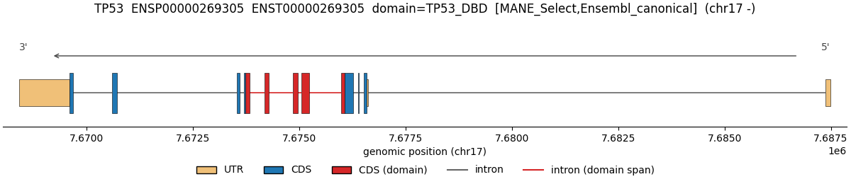
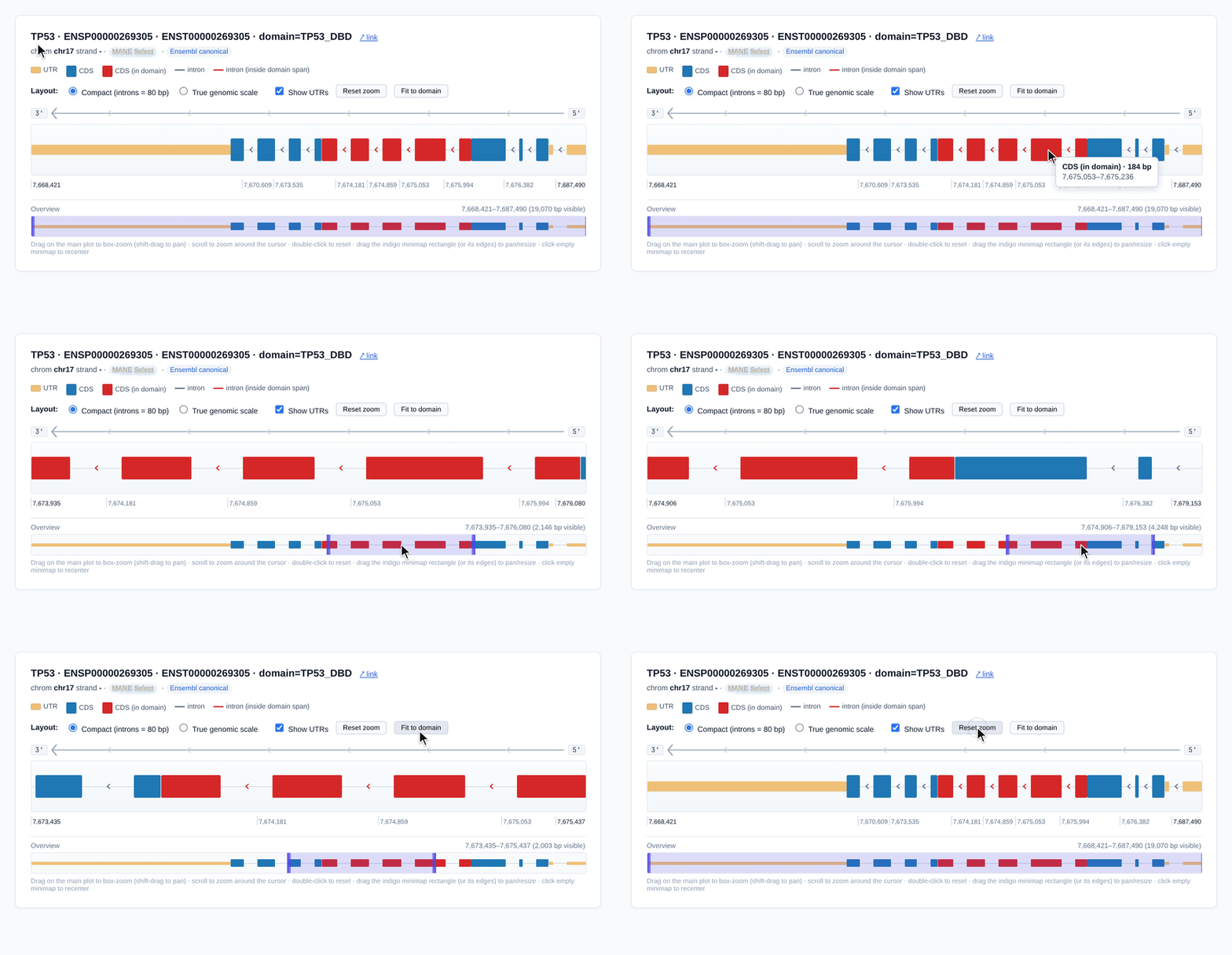
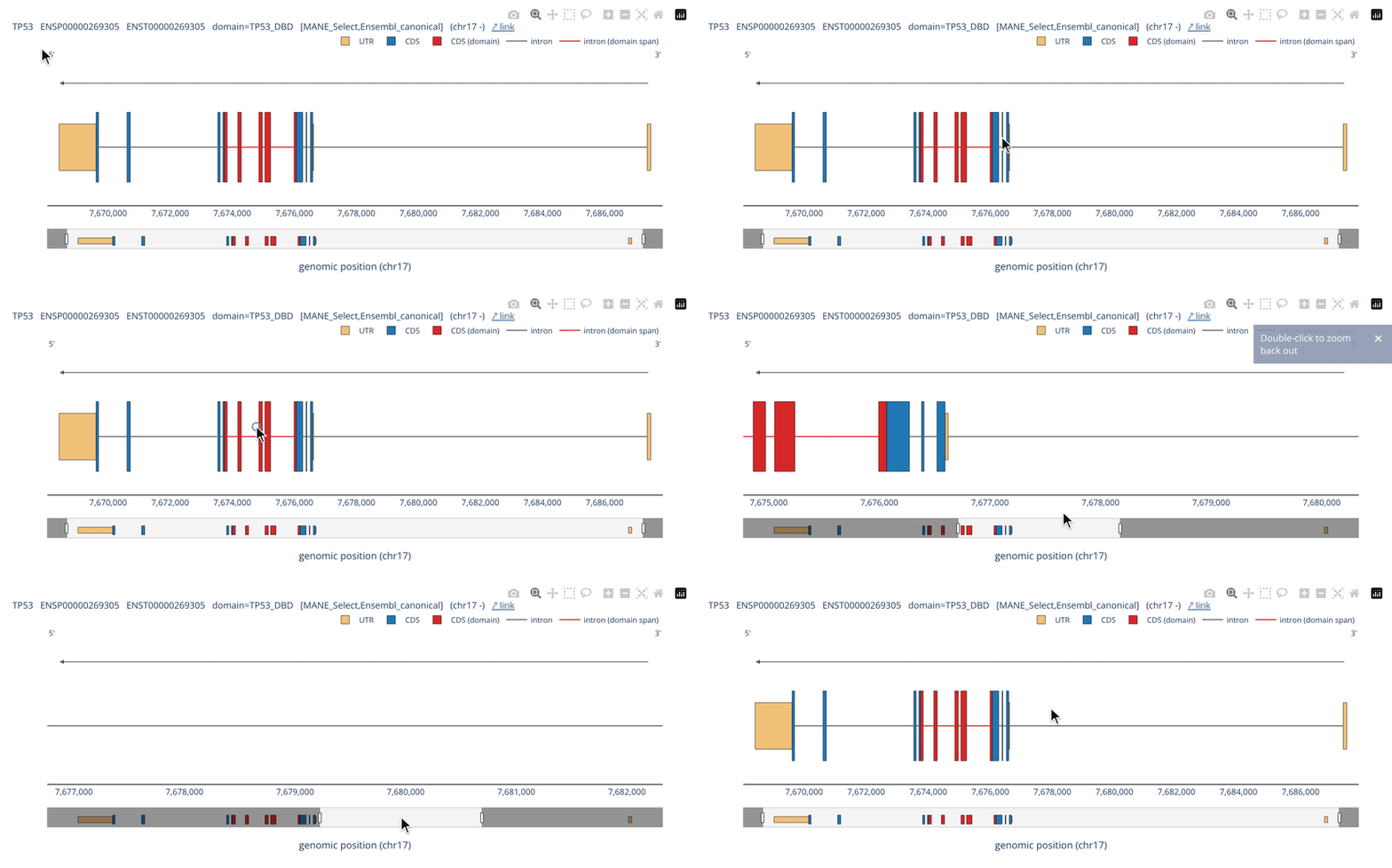
Same isoform (TP53, DBD highlighted), rendered three ways:

Type	Renderer	Command	Notes
Static	matplotlib	--out fig.pdf (or .png / .svg)	Publication-ready vector/raster; no interaction.
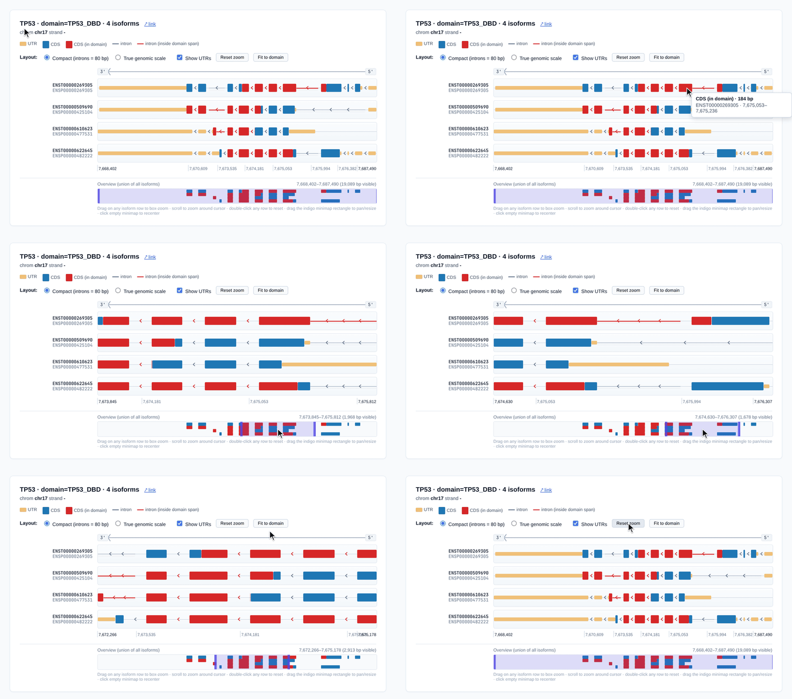
Interactive	vanilla JS (default)	--out fig.html	Self-contained (~40 KB), no dependencies, works offline: box-zoom, pan, wheel-zoom, draggable minimap.
	plotly	--out fig.html --engine plotly	Loads plotly.js from a CDN; hover tooltips and a bottom rangeslider.

Static (matplotlib)

Interactive, vanilla JS

Interactive, plotly

Multiple isoforms on one axis

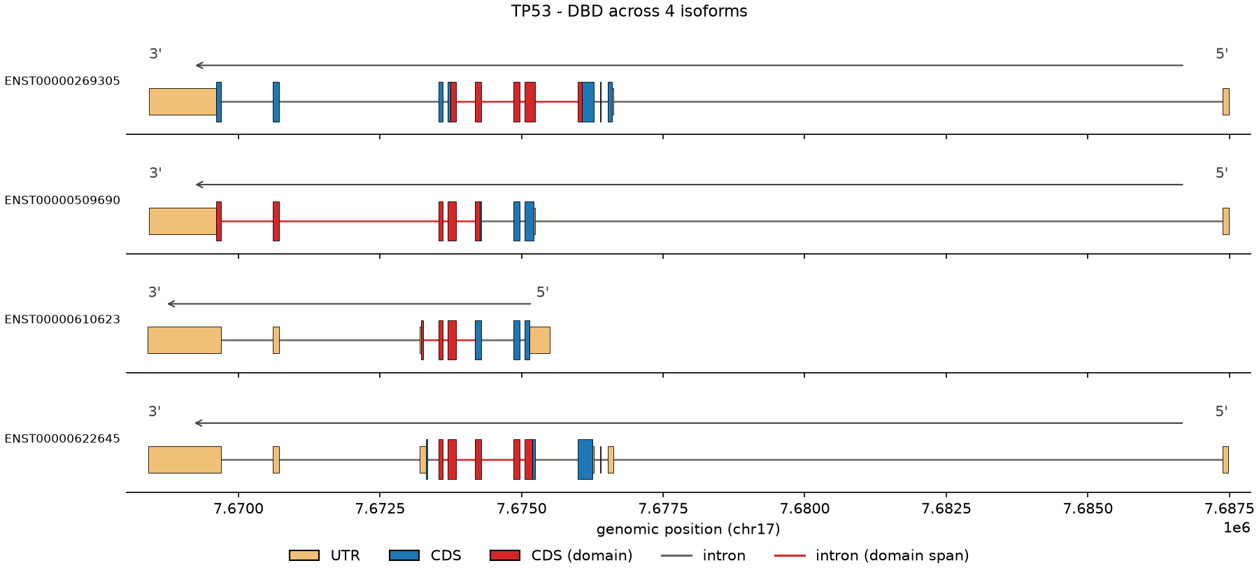
Every isoform of a gene on one shared genomic axis, with the queried domain marked red on each isoform that codes it. Available as a static matplotlib figure and as the interactive stack viewer (render_interactive_html_stack).

Static

Interactive

Static figures

CLI

Render a single query to a vector PDF:

fastCDS plot \
    --isoform results/isoform_structure.tsv \
    --input-id TP53_DBD \
    --out tp53.pdf

The output format follows the file extension (.pdf, .png, or .svg). To render every input_id in the TSV at once, use --all; with a .pdf target this becomes a single multipage PDF (one query per page), while a .png/.svg target writes one file per query named base.<input_id>.ext:

fastCDS plot --isoform results/isoform_structure.tsv --all --out queries.pdf   # multipage PDF
fastCDS plot --isoform results/isoform_structure.tsv --all --out queries.png   # queries.TP53_DBD.png, ...

Python

From a MappingResult (or an isoform DataFrame, or a path to the TSV):

import fastCDS as fc

result = fc.map_query("ENSP00000269305", aa_start=10, aa_end=50, domain_id="TP53_DBD", index="human.idx")
fc.plot(result, input_id="TP53_DBD", out="tp53.pdf")

fc.plot() returns the matplotlib Figure (useful when you pass neither out nor an HTML target). For batches, fc.plot_all(source, out="queries.pdf") mirrors --all. See Python API for the full client.

Arguments

Flag / kwarg	Default	Effect
--isoform FILE	required	Path to the isoform_structure.tsv to plot.
--input-id ID	-	Render a single query (mutually exclusive with --all).
--all	-	Render every input_id; multipage PDF if --out ends in .pdf, else one file per query.
--out FILE	required	Output file; the extension picks the format (.pdf/.png/.svg static, .html interactive).
--title STR	derived	Override the auto-generated title.
--width, --height	12, 2.6	Figure size in inches.
--no-highlight	off	Don't color CDS-in-domain segments red.
--no-introns	off	Hide intron lines.
--no-utr	off	Hide UTR boxes.
--spliced	off	Concatenate non-intron features in translation order (no introns).
--compact-genomic	off	Genomic order, but clamp each intron to a fixed display width (best for long-intron genes); CDS/UTR stay at true bp scale with a // compression mark. Mutually exclusive with --spliced.

The Python plot() / plot_all() functions accept the same toggles as keyword arguments (input_id, out, title, width, height, show_introns, show_utr, highlight_domain, spliced, compact_genomic).

Interactive viewers

CLI

An .html target renders the interactive viewer. --engine picks the renderer; its two values are js (the default - the self-contained vanilla-JS viewer) and plotly. So --out x.html alone gives you JS; --engine js is only needed if you want to be explicit:

# self-contained vanilla-JS viewer (no CDN, single offline file) - the default
fastCDS plot --isoform results/isoform_structure.tsv --input-id TP53_DBD --out tp53.html
# the title linkout is automatic from the ID; add --link-template 'URL' to override it
# identical to the first command, engine spelled out:
fastCDS plot --isoform results/isoform_structure.tsv --input-id TP53_DBD \
    --out tp53.html --engine js

# plotly engine (CDN-backed; hover tooltips and a bottom rangeslider)
fastCDS plot --isoform results/isoform_structure.tsv --input-id TP53_DBD \
    --out tp53.html --engine plotly

Both engines ship with pip install fastCDS. The standalone js viewer supports box-zoom (drag to zoom into a genomic range), shift-drag to pan, mouse-wheel zoom, double-click to reset, a draggable minimap, UTR rendering with strand arrows, and a Compact / True-genomic layout toggle. A clickable linkout next to the title is added automatically from the ID - Ensembl stable IDs (ENSP/ENST/ENSG) link to Ensembl, RefSeq (NP_/XP_/NM_/XM_) to NCBI, UniProt accessions to UniProt; custom-GTF IDs get no link. Pass --link-template to override it with your own URL, using the placeholders {protein_id}, {gene_name}, {transcript_id}, {chrom}, {start}, {end}.

With --all, an .html target writes one file per query (base.<input_id>.html).

Python

For a single isoform, obtain the segments from a result and embed the viewer inline in a notebook:

import fastCDS as fc

result = fc.map_query("ENSP00000269305", aa_start=10, aa_end=50, domain_id="TP53_DBD", index="human.idx")

fc.render_interactive_jupyter(result, input_id="TP53_DBD", plot_height=160)

For several isoforms stacked in one viewer, hand the whole result (or a TSV path) to the stack variant - every isoform in it is stacked:

fc.render_interactive_jupyter_stack(result, plot_height=40)

To write standalone HTML files instead of embedding inline, use the file builders fc.render_interactive_html(result, "tp53.html", input_id="TP53_DBD") and fc.render_interactive_html_stack(result, "stack.html"). See Tutorials and Notebooks for end-to-end notebook examples.

Arguments

Flag / kwarg	Default	Effect
--out FILE / out=	required	Output file; .html selects the interactive viewer.
--engine {js,plotly} / engine=	js	Interactive renderer for .html output. js = self-contained (no CDN, offline); plotly = CDN-backed, needs plotly. Ignored for static output.
--link-template URL / link_template=	auto	External linkout next to the title (.html only). Auto-derived from the ID by default (Ensembl / RefSeq / UniProt; none for custom IDs); pass a URL to override, with placeholders {protein_id}, {gene_name}, {transcript_id}, {chrom}, {start}, {end}.
--height N (CLI)	2.6	matplotlib figure height in inches (static path).
plot_height= (Python)	140 single / 40 stack	Main-track height in pixels for the Jupyter / standalone viewers.
height= (Python)	auto	Pin the Jupyter iframe height in px (for static exports where the auto-resize handshake can't fire).

The render_tfregdb2_* Python functions are deprecated aliases for the render_interactive_* names, kept only for backwards compatibility and slated for removal.