Radio Tomographic Imaging Tutorial

Interactive PyQt5 tutorial for Radio Tomographic Imaging (RTI). The app lets you draw an attenuation layout, define TX/RX movement paths, collect line-integral measurements, inspect the projection matrix, reconstruct the attenuation image, and experiment with segmentation methods.

This is an academic initiative from the Sensing and Networked Systems Engineering (SeNSE) Group at IIT Madras.

Features

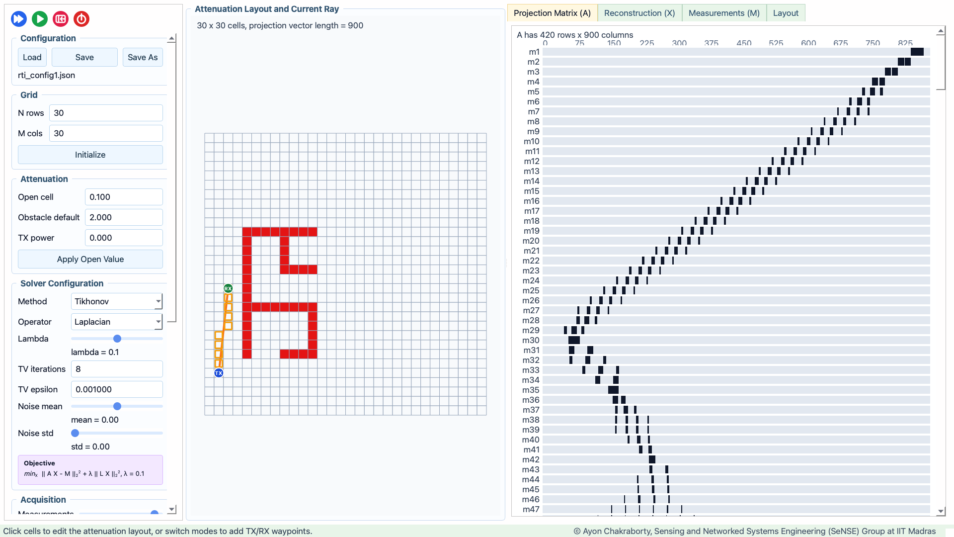
• Grid-based attenuation layout editor.
• TX and RX waypoint drawing with Bresenham ray tracing between current positions.
• Step-by-step or continuous measurement acquisition.
• Live projection matrix visualization.
• Reconstruction with least squares, Tikhonov regularization, and total variation IRLS.
• Noise controls for measurement mean and standard deviation.
• Segmentation playground for reconstructed layouts.
• JSON configuration loading and saving.

Screenshots

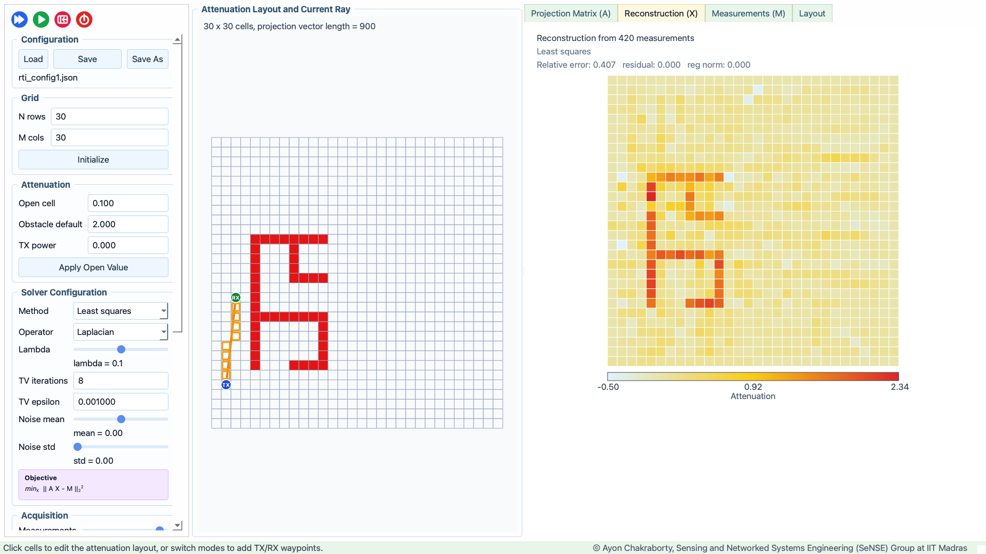
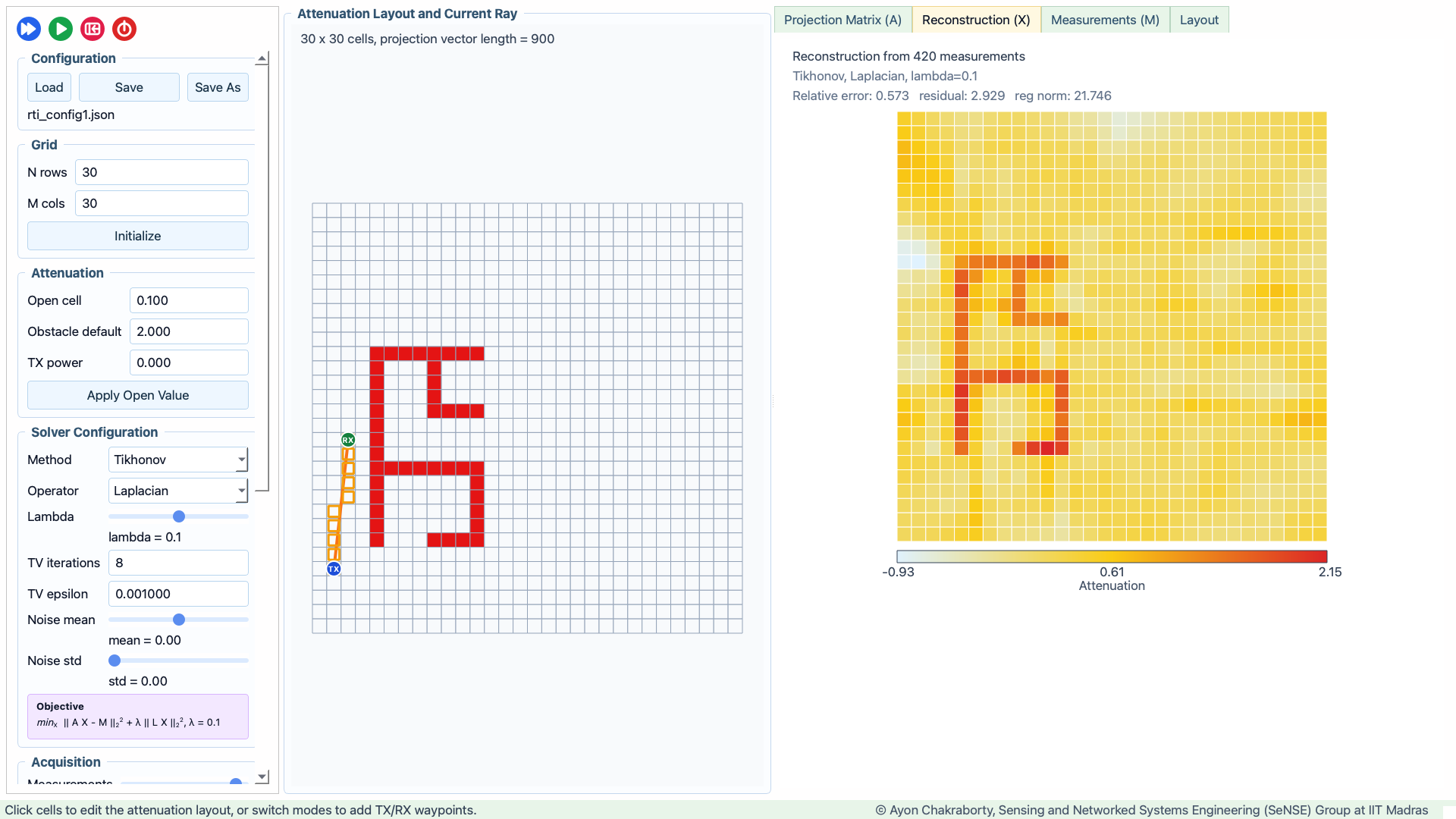
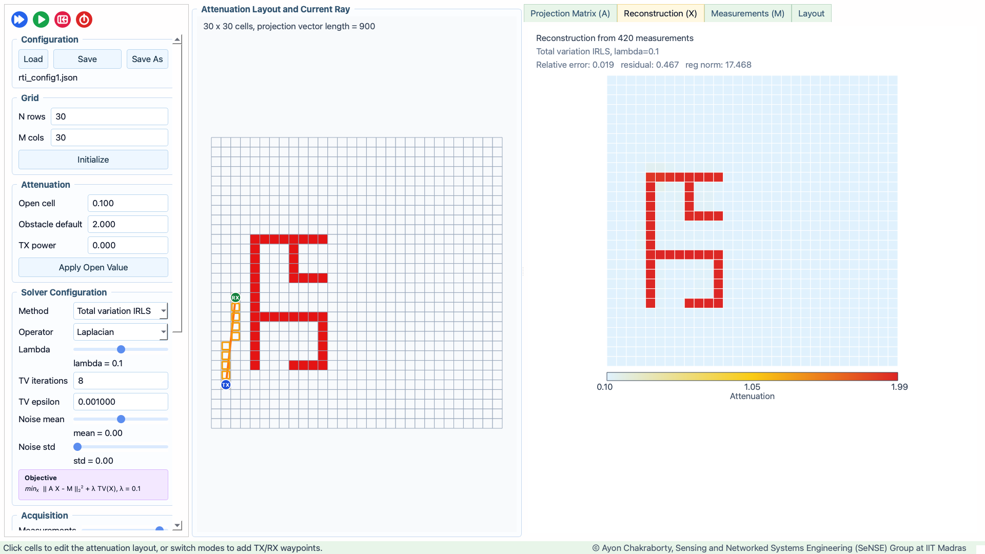
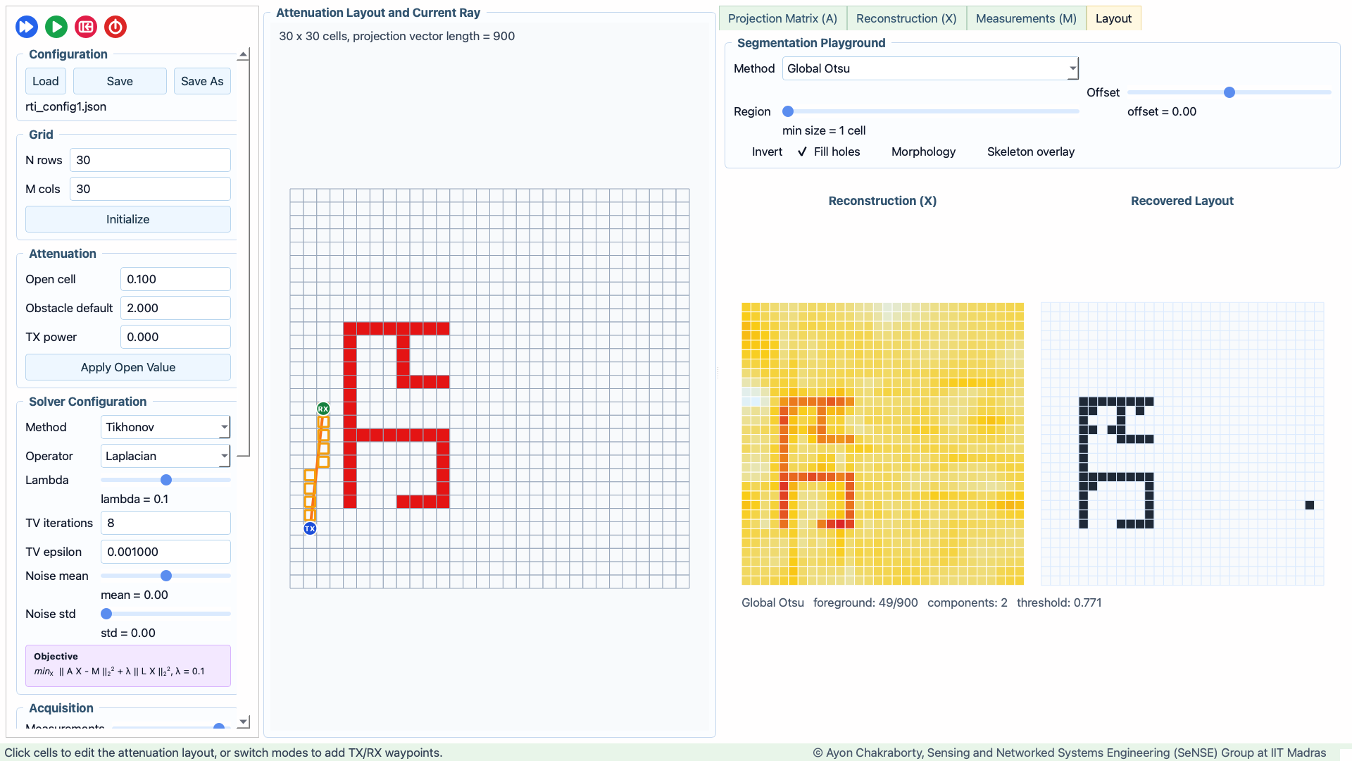
The screenshots below were captured from the Python window at 1920x1080 after loading configs/rti_config1.json and advancing to 420 measurements.

Projection Matrix

Least Squares Reconstruction

Tikhonov Reconstruction

Total Variation Reconstruction

Layout Thresholding

Project Layout

RTI_Tutorial/
├── configs/                  # Saved and sample RTI configuration JSON files
│   └── rti_config1.json
├── docs/
│   └── screenshots/          # README and documentation screenshots
├── src/
│   └── rti_tutorial/
│       ├── assets/           # Package screenshots used for PyPI/package assets
│       ├── config/           # Config load/save code
│       ├── core/             # RTI model, solvers, waypoint logic, segmentation
│       └── gui/              # PyQt windows, controls, widgets, workers
├── main.py                   # Local launcher
├── pyproject.toml            # Installable package metadata
└── requirements.txt          # Minimal runtime requirements

Setup

Use Python 3.10 or newer.

After the package is published on PyPI:

pip install rti-tutorial
rti-tutorial

For optional segmentation acceleration and OpenCV-based skeletonization:

pip install "rti-tutorial[segmentation]"

For local development from this repository:

python3 -m venv .venv
source .venv/bin/activate
pip install --upgrade pip
pip install -r requirements.txt

For editable package installation:

pip install -e .

Optional segmentation acceleration and OpenCV-based skeletonization:

pip install -e ".[segmentation]"

Run

From the project root:

python main.py

If installed with pip install -e ., you can also run:

rti-tutorial

If installed from PyPI, the same command launches the GUI:

rti-tutorial

Configuration Files

Configuration JSON files are stored in configs/. The included sample is:

configs/rti_config1.json

In the app, use Load to open this file. The Save As dialog defaults to the configs/ folder so new scenarios stay grouped with the sample configurations.

Each configuration stores:

• Grid dimensions.
• Open-cell and obstacle attenuation values.
• TX power and measurement noise settings.
• Obstacle mask and per-cell attenuation matrix.
• TX/RX waypoint paths.
• Solver method, regularization operator, and solver parameters.

The included sample has a 30 x 30 grid and 446 possible TX/RX trajectory positions. Load it, then use Run, Step, or the Measurements slider to move past 400 measurements and compare the reconstruction and thresholding algorithms on the same data.

Reconstruction Options

The Solver Configuration panel controls how the attenuation image X is reconstructed from the projection matrix A and measurement vector M.

• Least squares solves the direct inverse problem by minimizing ||A X - M||2^2. It is useful as a baseline and shows what the measurement geometry alone can recover.
• Tikhonov adds a regularization term, lambda ||L X||2^2, to stabilize the reconstruction. The operator selector can use identity, first-difference gradient, or Laplacian regularization.
• Total variation IRLS uses an iterative total-variation style penalty. It is useful when the expected layout has sharper boundaries and piecewise-smooth regions.
• Lambda controls regularization strength. Lower values follow the measurements more closely; higher values smooth or constrain the result more strongly.
• TV iterations and TV epsilon control the total-variation IRLS approximation.
• Noise mean and Noise std add deterministic simulated Gaussian measurement noise. The mean shifts the measurement loss, and the standard deviation controls spread. Changing either value regenerates the measurement vector for the current measurement count.

Layout Thresholding Options

The Layout tab turns the reconstructed attenuation image into an estimated obstacle layout. It includes several thresholding and segmentation choices:

• Global Otsu computes one threshold for the full reconstruction.
• Local Otsu computes thresholds over local windows so different parts of the grid can adapt independently.
• Manual Threshold lets you choose the threshold ratio directly.
• Adaptive Mean thresholds against a local mean plus an offset.
• RAG Regions quantizes the reconstruction into regions and reports region adjacency information.
• Morphology Cleanup applies thresholding followed by cleanup operations such as filling small gaps.
• Skeletonization extracts a thin structural representation of the thresholded layout.
• Gradient Edges emphasizes strong spatial changes in attenuation rather than filled obstacle regions.

The layout controls also include threshold offset, local window size, minimum region size, RAG levels, invert, fill holes, morphology cleanup, and skeleton overlay toggles.

Basic Workflow

1. Start the app with python main.py.
2. Load configs/rti_config1.json, or initialize a new grid.
3. Edit cells to mark obstacles and adjust attenuation values.
4. Switch to Draw TX and Draw RX modes to add movement waypoints.
5. Click Step or Run to collect measurements, or use the Measurements slider to jump to a specific count.
6. For the sample config, move to 400+ measurements and try least squares, Tikhonov, and total variation reconstruction.
7. Open the Layout tab and compare Otsu, local Otsu, adaptive mean, manual thresholding, morphology cleanup, skeletonization, and edge-based methods.
8. Save the scenario as a JSON file in configs/.

License

Copyright (C) 2026 Ayon Chakraborty, Sensing and Networked Systems Engineering (SeNSE) Group at IIT Madras.

This project is licensed under the GNU General Public License v3.0 or later. See LICENSE.

Development Checks

Syntax check all Python files:

python -m compileall main.py src

Quick config load smoke test:

python - <<'PY'
from pathlib import Path
import sys

sys.path.insert(0, "src")
from rti_tutorial.config.io import load_model_config

model = load_model_config(Path("configs/rti_config1.json"))
print(model.rows, model.cols, len(model.tx_waypoints), len(model.rx_waypoints))
PY

Expected output for the included sample:

30 30 64 94