
Alan Turing : Turing machine and Turing test
Neural Networks(Donald Hebb, 1949)
Perceptron(Frank Rosenblatt, 1958) <-> (Marvin Minsky, 1969)
Multiplayer Perceptron(1986)
SVM(1995)
Deep Neural Networks(Geoffrey Hinston, 2006)

- Unsupervised Learning : clustering, dimension reduction by Density estimation, Pretraining
- Supervised Learning : speech/face recognition by Classification, Regression
- Pattern Analysis(CSE@TAMU Gutierrez-Osuna) [slide]
- Semi-supervised Learning
- Reinforcement Learning : alphago, self-driving, machine translation
- credit assignment problem
- trade-off between exploration and exploitation
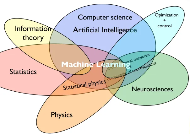
Data is given as a vector, matrix or tensor.
Everthing is probabilistic due to noise.
A single point does not say much, so statistics comes to rescue.
Seminar for Deep Learning:Learning Based on deep neural network [slides]
Object : 학습 데이터를 이용하여 모델을 근사한 후, 임의의 입력 데이터 x에 대해 예측결과 t를 제공
- Probablility Theory : 불확실성을 정량화시켜 표현할 수 있는 수학적인 프레임워크를 제공
- Decision Theory : 확률적 표현을 바탕으로 적절한 기준에 따라 최적의 예측을 수행할 수 있는 방법론을 제공
1) Task1 : 모델링할 함수를 알아내기 위해 이를 근사할 수 있는 근사(Approximate)식이 필요하다.
- Tayler seires : 차수(M)을 늘릴수록 특정 위치에서의 함수를 잘 근사. 일반화에는 약간 거리가 있음 [blog]
$$f(x) = f(a) + f'(a)(x-a) + \frac{f''(a)}{2!}(x-a)^2 + \frac{f'''(a)}{3!}(x-a)^3 + \ldots$$ - 퓨리에 변환식
$$F(w) = \int_{-\infty}^{\infty} f(t)e^{-iwt}dt$$
2) Task2 : 식을 근사하기 위해
- 에러 함수(Error Function) : 제곱합(sum-of-squares) 에러 함수를 주로 사용
$$E(w) = \frac{1}{2}\sum\limits_{n=1}^N ({y(x_n,w)-t_n})^2$$
3) Task3(model selection) : 최적의 차수(M)의 개수를 찾는다. M이 너무 작으면 under-fitting, 너무 높으면 over-fitting 현상이 발생한다.
4) Task4 : 모델의 평가를 위해 에러 값의 정도를 수치화한다.
- N으로 나누는 것은 데이터셋 크기가 다른 스케일 문제를 보정하기 위한 정규화(Normalization) 요소임
5) Task5 : Over-fitting 문제를 해결한다.
- 관찰 데이터의 크기가 클수록 over-fitting 현상이 줄어든다. 그러나 휴리스틱 관점에서, 모델 파라미터 개수(M)는 샘플 크기의 1/5, 1/10 정도보다 작은 것이 좋다.
- Regularization : w값의 범위를 제한하여 모델의 복잡도(M,차수)는 올리면서 over-fitting을 막아내는 것
$$E(w) = \frac{1}{2}\sum\limits_{n=1}^N ({y(x_n,w)-t_n})^2+\frac{\lambda}{2}||w||^2 \ (||w||^2 = w^Tw)$$ - MLE, Bayesian 등으로 적절한 M 값을 찾아내는 방식도 존재함
불확실성을 정량화시켜 표한할 수 있는 수학적인 프레임워크를 제공한다.
불확실성(Uncertainty)은 데이터 크기의 부족 혹은 노이즈(Noise)로 인해 발생한다.
확률의 법칙
- sum rule :
$p(X) = \sum\sigma_{Y} p(X,Y)$ - product rule :
$p(X,Y) = p(Y|X)p(X)$ (if - Bayesian rule :
$p(Y|X) = \frac{p(X|Y)p(Y)}{p(X)}$ [blog]
밀도 추정(Density Estimation) : 주어진 데이터x로부터 확률 밀도 함수(probability density function, PDF)를 추정하는 과정 - unsupervised
- 확률이 이산(discrete)적인 사건
- Histogram
- PMF(Probability Mass Function) : 각 데이터 포인트에 대한 상대 빈도를 계산
- 확률이 연속일 경우
- KDE(Kernel Density Estimation) : 확률값을 구간(range)로 표현한다. 구간 적분해야 확률값이 된다.
- 평균(Expactation)
-
$E[f] = \sum_x p(x)f(x)$ (이산) -
$E[f] = \int p(x)f(x) dx$ (연속)
-
- 조건부 평균(기댓값) :
$E_x[f|y] = \sum_x p(x|y)f(x)$ - 분산(variance) :
$var[f] = E[f(x) - E[f(x)])^2] = E[f(x)^2] - E[f(x)]^2$ - 임의의 변수 x,y에 대한 공분산(covariance)
- cov[x,y] = E_{x,y}[(x - E[x])(y - E[y])] = E_{x,y}[xy] - E[x]E[y] (실수)
- cov[x,y] = E_{x,y}[(x - E[x])(y^T - E[y^T])] = E_{x,y}[xy^T] - E[x]E[y^T] (벡터)
- distributions
- uniform : continous variable
- Bernoulli : binary variable
$E[x]=p \quad var[x] = p(1-p)$ - binomial : N times
$var[m] = Np(1-p)$ - categorical : bernoulli to K-dim binary variable
- multinomial
- Laplacian : ㅅ shape
- beta and dirichlet :
실제 측정된 빈도수에 따라 확률을 계산하는 Frequentism과 다르게 Baysianism은 믿음의 정도로 불확실성을 정량화할 수 있다. MLE(Maximun Likelihood Estimation)과 달리, 파라미터 w를 랜덤변수로 간주하여 확률분포를 사용한다.
- 2개의 파리미터(모수,parameter) :
$\mu$ :평균(mean),$\sigma$ :표준편차(standard deviation) - 정확도(precision) : 분산(표준편차 제곱)의 역수
$\beta = \frac{1}{\sigma^2}$ - 가우시안 분포, 즉 정규분포의 장점은 1차원의 속성을 D차원으로 확장 가능하다는 것이다. 이를 다변량(multinominal) 가우시안 분포라고 부른다.
$$N(x|\mu, \Sigma) = \frac{1}{(2\pi)^{D/2}|\Sigma|^{1/2}} exp(-\frac{1}{2}(x-\mu)^T\Sigma^{-1}(x-\mu)) (\Sigma:covariance:DxD)$$ - 주어진 데이터가 어떤 가우시안 분포를 따르는지 해를 구하려면 평균과 분산(파라미터)를 추정하면 된다.
$$\mu_{MLE} = \frac{1}{N} \sum\limits_{n=1}^N x_n \quad \sigma_{MLE}^2 = \frac{1}{N} \sum\limits_{n=1}^N {(x_n - \mu_{MLE})}^2$$ - MLE에서 발생하는 over-fitting의 한 예는 분산값의 bias이다.
모집단의 샘플 그룹들에 대해 각각의 평균 값을 평균하면 실제 평균값과 가까워진다. 그러나 각각의 분산 값을 평균해도 실제 분산 값에 가까워지진 않는다.

multi-modal D차원 상의 데이터는 N번 관찰 시 V크기의 부피공간 영역R에 속하는 데이터의 수K로 확률밀도함수p(x)를 표현할 수 있다.
-
KDE(Kernel Density Estimators) : V를 고정시키고 K를 결정
- 커널 함수(kernel method) : 임의의 한 점 x가 주어졌을 때, 각 차원으로 h 거리 내(Parzen Window)에 존재하는 모든 샘플을 센다 - 아직은 discontinuous
- smoothing : 연속적인 확률분포를 구성하기 위해 하나의 샘플
$x_n$ 에 대해 중심이$x_n$ 이고 표준편차가 h인 정규분포(smooth kernel)를 만들고 이를 합하여 새로운 밀도함수를 만들어내는 것. - h값이 충분히 크지 않으면 under-smooth, 충분히 작지 않으면 over-smooth가 발생한다.
-
KNN(K-NEarest Neighbors) : K를 고정시키고 V를 결정
- 샘플 데이터
$x_n$ 을 중심으로 하는 구(sphere)가 K개의 샘플을 포함할 때까지 구의 반지름을 늘려, 구의 부피V와 확률밀도p(x)를 구한다. - 주로 분류(classification) 문제에 사용된다.
- K값으로 smoothing 정도를 조절할 수 있다.
- 샘플 데이터
- mixture of Gaussian : clustering
정보(information) : "학습에 있어 필요한 놀람의 정도(degree of surprise)"
- 밑수가 2라면 정보량의 단위는 bit라고 보면 된다. 밑수는 무엇이든 될 수 있다.
- Non-Uniform 분포의 엔트로피는 Uniform 분포의 엔트로피보다 낮다.
ex) a,b,c,d,e,f,g,h 8글자의
확률분포가 동일($\frac{1}{8}$ )할 경우 :$H[x] = -8 * \frac{1}{8}log_2\frac{1}{8} = 3 bits$
확률분포가 ($\frac{1}{2} , \frac{1}{4} , \frac{1}{8} , \frac{1}{16} , \frac{1}{32} , \frac{1}{64} , \frac{1}{64}$ )일 경우 :
$H[x] = -\frac{1}{2}log_2\frac{1}{2} - \frac{1}{4}log_2\frac{1}{4} - \frac{1}{8}log_2\frac{1}{8} - \frac{1}{16}log_2\frac{1}{16} - \frac{1}{32}log_2\frac{1}{32} - \frac{1}{64}log_2\frac{1}{64} - \frac{2}{128}log_2\frac{1}{128}= 2bits$
$E[length] = \frac{1}{2} * 1 + \frac{1}{4} * 2 + \frac{1}{8} * 3 + \frac{1}{16} * 4 + \frac{1}{32} * 6 + \frac{1}{64} * 6 + \frac{1}{128} * 6 + \frac{1}{128} * 6 = 2 bits$
(hoffman code : 0, 10, 110, 1110, 111100, 111101, 111110, 111111)
즉, 엔트로피는 랜덤 변수의 상태를 전송하는데 필요한 비트 수의 Lower Bound이다.
통계역학 관점에서 엔트로피는 "어떤 계의 무질서도" 도는 "거시 상태에 대응되는 미시 상태의 가짓 수"로 표현된다.
최대 엔트로피 값을 구하기 위해 라그랑지안 승수(제약 조건 상에서 함수의 최소값을 찾는 수단)을 사용한다. [blog]
- 미분 엔트로피(differential entropy)
- 입력 변수가 연속일 때, 가우시안 분포가 entropy를 최대로 만든다
- 입력 변수가 이산일 때, 균일(uniform) 분포가 엔트로피를 최대로 만든다.
- 조건부 엔트로피(conditional entropy)
mutual information : y를 알고 난 후에 x의 불확실성을 줄이는 과정 - 연관 엔트로피(Relative entropy)
- Relative Entropy 또는 KL(Kullback-Leibler) divergence : digergence between two probability distributions p and q
$$KL(p||q) = - \int p(x)ln(\frac{q(x)}{p(x)}) dx = (cross-entropy) - (entropy-of-x)$$ 
- Jensen's Inequality for convex function [blog]
$$\ if\ \phi(E[X]) \leq E[\phi(X)] , \phi(x)\ is\ convex$$ 즉, KL divergence를 최소화하는 것은 likelihood(가능도 함수)를 최대화 시키는 것과 동일하다 -> MLE와 연관성을 지님
- Relative Entropy 또는 KL(Kullback-Leibler) divergence : digergence between two probability distributions p and q
확률적 표현을 바탕으로 적절한 기준에 따라 최적의 예측을 수행할 수 있는 방법론을 제공한다.
- Generative Model : 데이터 생성과정을 모델링하여 분포를 학습하여 used for classification by the Bayes' rule
$$p(t|x) = \frac{p(x|t)p(t)}{p(x)}$$ - Discriminative Model : 클래스 레이블을 학습하여 결정 경계를 찾아내 just for classification
$p(t|x)$ - Discrimination Function : model of map function
- Minimize misclassification rate

$$p(mistake) = \int_{R_1} p(x,C_2)dx + \int_{R_2}p(x,C_1)dx = 1 - \sum\limits_{k=1}^K \int_{R_k}p(x,w_k)dx)$$ - Minimize expected loss(Loss function, know as Cost function) : 하나의 샘플x가 실제로는 특정 클래스
$C_k$ 에 속하지만, 모델이 이 샘플의 클래스를$C_j$ 로 선택할 때 들어가는 비용을 정의$$E[L] = \sum_k\sum_j\int_{R_j}L_{kj}p(x,C_k)dx$$ - Mean Squared Error
$\frac{1}{N}\sum\limits_{i=1}^N(t_i-y_i)^2$ - Cross Entropy : classification 문제에 사
- Hinge Loss : svm 모델에 사용
$max(0,1-ty)$
- Mean Squared Error
- Accuracy =
$\frac{(TP+TN)}{Total}$ : 맞게 판단한 비율 - Precision =
$\frac{TP}{(TP+FP)}$ : 진짜라고 한 것 중 진짜인 비율 - Recall =
$\frac{TP}{(TP+FN)}$ : 진짜들 중 진짜인 비율 - F1 score =
$\frac{2PR}{(P+R)}$ : harmonic mean of Precision and Recall - Area Under the roc(TPR/FPR) Curve : perfect=1, random=0.5

Unsupervised Learning : only input
- clustering : grouping samples in a way that samples in the same group are more similar to each other than to those in other groups
- How to measure the similarity?
- How many clusters?
- Hierarchical Clustering
- bottom-up : merge the closest(nearest/average/fareast) groups one by one until the number of cluster of cohesion threshold
- top-down
- kMeans
- k개의 중심점을 랜점으로 초기화 -> 클러스터에 데이터 합류 -> 클러스터 평균을 계산해 중심접 업데이트
- 초기 중심 선택에 종속적이며 distance function이 중요하다. outlier들에 민감하다.
- k개의 중심점을 랜점으로 초기화 -> 클러스터에 데이터 합류 -> 클러스터 평균을 계산해 중심접 업데이트
- MoG(Mixture of Gaussian, known as GMM) : a distribution can be approximated by a weighted sum of M components Gaussian densities
- parameters : {
$\pi_i, \mu_i, \Sigma_i$ }

- EM : since Z in unknown, we want to maximize the expectation of log probability (joint probability or likelihood) across all possible Z
in EM, it uses the distribution of hidden variables Z instead of using the best Z - Expectation step : estimate parameters using Lagrange multiplier, considering no prior

- Maximization step : maximize the posterior probability(or likelihood)

- parameters : {
More features porived more informaation and potentially high accuracy
but make harder to train a classifier(curse of dimensionality)
with increasing the possibility of overfitting
=> DR(Finds continuous latent variable, like Z) could be a rescue
- PCA is a linear projection of the data onto a lower dimension space z
- minimal reconstruction error(RSS:residual sum of square) :
$||x - \overset{~}{x}||$ - maximal preserved variance
- PPCA(Probabilistic PCA) : (gaussian distribution)probabilistic model of PCA for the observed data
- maximum-likelihood parameter estimates
- generative view : sampling x conditioned on the laten value z
- FA and PCA
- PCA transforms the obsrevations to a new space with the larger variance
- FA describes observations in term of latent variable, factors
- MDS(Multi-dimentional scaling)
extensions from PCA to supervised learning(classification)

Objective : maximize the ratio of the variance between classes to the one within the classes on the projected space
extensions from PCA to independent factors

decompose given multivariate data into a linear sum of statistically independent components
Objective : max likelihood, max nonGaussianity, min/mutual informatin
constraint : W and H can not have negative value
RBM
Supervised Learning : classification and regression both
- classification : predicting a discrete label of input(interested in the boundary of classes)
- regression : predicting the quantity of output(interested in the relationship of input and output)
- data and label
- training/valid/test sets
- cross-validation : split the data into training(including validation) and testing
random subsampling, K-fold, leave-one-out, etc - approach for overfitting : more data samples, simpler model, regularization methods, early stopping
- pros
- no conditional costs for training (:lazy memory-based learning)
- easy to implement
- converges to optimal calssifier
- cons
- higher computational costs for testing
- greater storage requirements
- curse of dimensionality
- Solve
- approximation for speed-up : bucketing, k-d tree(select an randome axis to construct k-d trees)
- proper k needs to avoid under/over-fitting
- DT is a tree-shaped prediction model : sequence of questions = non-metric method without a measure of distance between features
- prediction : how can we predict new data?
- training : how could we select odd branch?
- Gini impurity(used in CART) measures how often a decision would be incorrect if it was randomly labeled according th the distribution of labels in the subset. $$$GI = 1 - \sum\limits_i^c \pi^2 dx$$
- Information Gain(used in ID3, C4.5) calculates the decrease in entropy after the dataset is split on a feature
$$IG = H(T) - H(T|a)$$ The highest IG is selected to split - Importance of node
$n$ = $p_nGI_n - p_{ln}GI_{ln} - p_{rn}GI_{rn} - pros
- simple to understand, interpret and visualize
- little effort is required for data preparation : normalization is not required
- able to obtain non-linear decision boundaries
- can handle both numeric and categorical data
- cons
- overfitting
- high variance(less stable)
- not able to extrapolate : can not apply to new sample data
ensemble learning method by consturcting a set of decision tree
An ensemble of classifiers is a aset of classifiers. They take simple algorithms and transform them into a super classifier without requireing any new algorithm
- bagging(or Boostrap Aggregating) : try model parallel and combine them
variance reduction - boosting : sequentially combine multiple base calssifiers(weak learners)
bias reduction ex) AdaBoost - Stacking : use the prediction of models as a training data
- Mixture of Experts : locally work experts got a seperate task
To predict the target y given a D-dimensional vector x
or to estimate the relationship between x and y
or to find the function from x to y
(x:independent variable, features, predictors / y:dependent variable, outcome)
To model categorical/continuous variables
- multinomial logistic regression(softmax regression)