Cones

Let $X$ be a vector space. A set $K \subseteq X$ is a convex cone if and only if

1. $x+y \in K$ for every $x,y \in K$ holds
2. $\lambda x \in K$ for every $\lambda \geq 0$ and $x \in K$

This notion is surprisingly versatile. A very simple cone is visualized in the following figure:

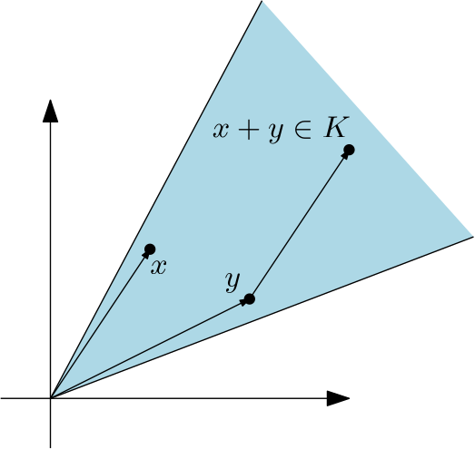
In CaΣoS, all cones have a shorthand.

Vector Cones

A vector cone is a set $K \subseteq \mathbb R^n$ for some $n \in \mathbb N$ (the dimension).

First-order Cone

The most simple examples of convex cones are linear subspaces of $\mathbb{R}^n$ as they appear in linear programming and even the positive orthant $\mathbb{R}^n_{\geq0}$.

Second-order Cone

The $n$-dimensional second-order (also quadratic or Lorentz) cone is defined as the set

$$\mathcal{Q}^n = \left\lbrace x \in \mathbb{R}^n \mid x_1 \geq \sqrt{x_2^2+x_3^2 + \dots + x_n^2 } \right\rbrace.$$

In three dimensions, the second-order cone resembles an ice cream cone, illustrated in the following figure of a cone in three variables:

Rotated Second-order Cone

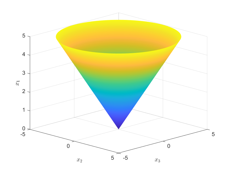
The $n$-dimensional rotated second-order (also quadratic or Lorentz) cone is defined as the set

$$\mathcal{Q}_{\text{rot}}^n = \left\lbrace x \in \mathbb{R}^n \mid 2x_1x_2 \geq x_3^2 + \dots + x_n^2 ,~ x_1,x_2 \geq 0 \right\rbrace .$$

Matrix Cones

A matrix cone is a subset of the space of symmetric matrices $\mathbb S_n \subset \mathbb R^{n \times n}$ for some $n \in \mathbb N$.

Positive Semidefinite Matrices

One concept that is particularly important to conic programming is the convex cone of all (symmetric) positive semidefinite matrices, defined as the set

$$\mathcal{S}^n_+ = \left\lbrace A \in \mathbb{R}^{n \times n} \mid \, A = A^{\top}, \, x^{\top} A x \geq 0 \, \text{ for all } x \in \mathbb{R}^n \right\rbrace$$

Consider for example the matrix $M\in\mathbb{S}^2$

$$M = \begin{bmatrix}x && y \\ y && z\end{bmatrix}$$

which is positive semidefinite for values of 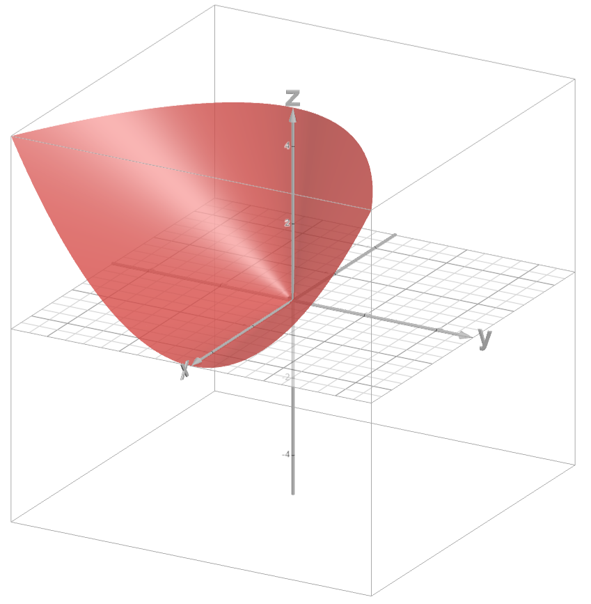$(x,y,z) \in \mathbb R^3$ that lie in the following cone:

The set of positive semi-definite is a closed convex set.

Diagonally Dominant Matrices

A symmetric matrix $A=(a_{ij})$ is diagonally dominant if

$$\forall i: a_{ii} \geq \sum_{j\neq i} |a_{ij}|$$

We denote the set of all diagonally dominant matrices as $\mathcal{DD}^n$.

Scaled Diagonally Dominant Matrices

A symmetric matrix $A=(a_{ij})$ is scaled diagonally dominant if there exists a diagonal matrix $D$, with positive diagonal entries, such that $DAD$ is diagonally dominant.

We denote the set of all scaled diagonally dominant matrices as $\mathcal{SDD}^n$.

Note

A relevant inclusion relationship between the cones of positive semidefinite matrices, diagonally dominant matrices, and scaled diagonally dominant matrices is

$$\mathcal{DD}^n \subseteq \mathcal{SDD}^n \subseteq\mathcal{S}^n_+$$

Polynomial Cones

A polynomial cone is a subset of the space of polynomials $\mathbb R[x]$.

Sum-of-Squares Polynomials

A multivariate polynomial $p(x)$ is sum of squares (SOS) if and only if it admits a representation

$$p(x) = \sum_{i=1}^m q_i(x)^2$$

where $q_i(x)$ are polynomials.

Notably, a polynomial $p(x)$ of degree at most $2d$ is SOS if and only if it can be written as

$$p(x) = [x]_d^{\top} Q [x]_d$$

where $Q$ is a positive semidefinite matrix and $[x]_d$ is the vector of all monomials of degree at most $d$.

Diagonally-dominant Sum-of-Squares Polynomials

A polynomial $p(x)$ of degree at most $2d$ is diagonally-dominant sum of squares (DSOS) if and only if it admits a representation

$$p(x) = [x]_d^{\top} Q [x]_d$$

where $Q$ is a diagonally dominant matrix and $[x]_d$ is the vector of all monomials of degree at most $d$.

Scaled-diagonally-dominant Sum-of-squares Polynomials

A polynomial $p(x)$ of degree at most $2d$ is scaled-diagonally-dominant sum of squares (SDSOS) if and only if it admits a representation

$$p(x) = [x]_d^{\top} Q [x]_d$$

where $Q$ is a scaled diagonally dominant matrix and $[x]_d$ is the vector of all monomials of degree at most $d$.

Conic modeling

We can use the conic framework to rewrite several typical convex sets in terms of conic quadratic formulations. Here are some examples:

Absolute values

For a constraint

$$|x| \leq c_1$$

we can use the definition of the two-dimensional quadratic cone where

$$x_1 \geq \sqrt{x_2^2}$$

needs to hold. Consequently, the constraint on the absolute value can be rewritten as

$$(c_1,x) \in \mathcal{Q}^2$$

Euclidean norm

In the standard definition of an $n$-dimensional quadratic cone

$$\mathcal{Q}^n = \left\lbrace x \in \mathbb{R}^n \mid x_1 \leq \sqrt{x_2^2+x_3^2 + \dots + x_n^2 } \right\rbrace$$

the right hand side of the inequality clearly provides the Euclidian norm of

$$\begin{bmatrix} x_2 & \dots & x_n \end{bmatrix}^{\top}.$$

That makes it possible for us to rewrite the inequality

$$\| x\|_2 \geq c_2$$

as

$$(c_2, x) \in \mathcal{Q}^{n+1}.$$

Cones in CaΣoS

All conic and sum-of-squares optimization interfaces expect the user to specify the cones of decision variables and constraints as structures within the option structure. To that extent, each cone type has a shorthand. A structure K describing the cones then consists of fields for each cone type to which the parameters describing the cone(s) are assigned. Cones of dimension zero can be omitted.

Shorthands for cone types

This list describes the shorthands and parametrization for the cone types described above.

Shorthands for vector and matrix cones

• K.lin : number of element-wise constraints;
• K.lor : vector $(d_1, \ldots, d_k)$ of second-order (Lorentz) cone dimensions;
• K.rot : vector $(d_1, \ldots, d_k)$ of rotated second-order (Lorentz) cone dimensions;
• K.sdp : vector $(s_1, \ldots, s_k)$ of positive semidefinite matrix cone dimensions, that is, $\mathcal K = \mathbb S_{s_1}^{+} \times \cdots \times \mathbb S_{s_k}^{+}$; the total number of SDP cone constraints is equal to $\sum_i s_i^2$;
• K.dd : vector $(s_1, \ldots, s_k)$ of diagonal dominant matrix cone dimensions;
• K.sdd : vector $(s_1, \ldots, s_k)$ of scaled diagonal dominant matrix cone dimensions.

Shorthands for polynomial cones

• K.lin : number of coefficient-wise constraints;
• K.sos : number of sum-of-squares constraints;
• K.dsos : number of diagonally-dominant sum-of-squares constraints;
• K.sdsos : number of scaled-diagonally-dominant sum-of-squares constraints.

Example

Consider Problem CQ01 from the Mosek Documentation:

$$\begin{align*} \text{minimize} \quad & x_4 + x_5 + x_6 \\\ \text{subject to} \quad & x_1 + x_2 + 2x_3 = 1, \\\ & x_1, x_2, x_3, x_5, x_6 \geq 0, \\\ & x_4 \geq \sqrt{x_1^2 + x_2^2}, \\\ & 2x_5 x_6 \geq x_3^2 \end{align*}$$

which can be solved with CaΣoS using the high-level interface (sdpsol).

We start off by defining $x\in \mathbb{R}^6$ as a CasADi symbolic variables with

x = casadi.SX.sym('x',6);
sdp.x = x;

Now we can define the cost function with

sdp.f = x(4) + x(5) + x(6);

All constraints now need to be defined in a vector:

sdp.g = [
    x(1) + x(2) + 2*x(3); % linear constraints come first
    [x(4); x(1); x(2)]; % In quadratic cone
    [x(5); x(6); x(3)]; % In rotated quadratic cone
]

where we need to define element-wise constraints first. Note that the right hand side of the element-wise constraint needs to be added using bounds:

lbg = 1;
ubg = 1;

The second row in sdp.g stems from

$$x_4 \geq \sqrt{x_1^2 + x_2^2}.$$

This can be rewritten as a conic constraint

$$\begin{bmatrix} x_4 \\ x_1 \\ x_2 \end{bmatrix} \in \mathbb{Q}^3$$

i.e. the $3$-dimensional quadratic cone. The order of the variables is crucial.

The third row describes the constraint

$$2x_5 x_6 \geq x_3^2$$

Since $x_5, x_6 \geq 0$, we can use the definition of the rotated quadratic cone to rewrite the constraint to

$$\begin{bmatrix} x_5 \\ x_6 \\ x_3 \end{bmatrix} \in \mathcal{Q}^3_{\text{rot}}.$$

Finally, we need to tell CaΣoS which cone should be used for each column of sdp.g.

opts.Kc = struct('lin', 1, 'lor', 3, 'rot', 3);

Additionally, we need to define linear bounds to the decision variable

opts.Kx = struct('lin', 6);
lbx = [0;0;0;-inf;0;0];
ubx = inf(6, 1);

which now allows us to define the solver and obtain the solution

% solver
S = casos.sdpsol('S','mosek',sdp,opts)

% solution
sol = S('lbx',lbx,'ubx',ubx,'lbg',lbg,'ubg',ubg);

Complete code:

% example see 
% https://docs.mosek.com/latest/toolbox/tutorial-cqo-shared.html

x = casadi.SX.sym('x',6);

sdp.x = x;
sdp.f = x(4) + x(5) +x (6);
sdp.g = [
    x(1) + x(2) + 2*x(3);
    [x(4); x(1);x(2)];
    [x(5); x(6);x(3)];
];

% cones
opts.Kc = struct('lin', 1, 'lor', 3, 'rot', 3);
opts.Kx = struct('lin', 6);

% solver
S = casos.sdpsol('S','mosek',sdp,opts)

% bounds
lbx = [0;0;0;-inf;0;0];
ubx = inf(6, 1);
lbg = 1;
ubg = 1;

% solution
sol = S('lbx',lbx,'ubx',ubx,'lbg',lbg,'ubg',ubg);