Multiple lattices

Multi-lattice Processing Tutorial (DUI2)

Introduction

This tutorial covers processing a dataset containing two overlapping crystal lattices using DIALS via DUI2. It is structured in three chapters:

• Discover — process as a single-lattice dataset first, use DUI2's visualisation tools to diagnose the second lattice, then re-index with max_lattices=5 and split the history tree into two independent branches
• Process — follow each branch through Bravais settings, refinement, and integration independently
• Post integration — scale and export each lattice independently

If you have not yet worked through a single-lattice dataset in DUI2, it is worth doing that first — this tutorial focuses on where the workflow diverges and why.

The dataset is a semi-synthetic two-lattice trypsin dataset collected at beamline I04, Diamond Light Source, available from Zenodo.

Download the data: semisynthetic_multilattice_data_2.tar.bz2

---

Chapter 1: Discover

The goal here is to run standard single-lattice processing as far as indexing, use DUI2's visualisation tools to confirm that a second lattice is present, then re-index with multi-lattice settings and split the tree.

1. Import images

When DUI2 starts, an incomplete dials.import node is already highlighted in the history tree. Click "Open images", navigate to the image directory, and select one CBF file. Click Run. The log confirms 100 images interpreted as a single sweep, written to imported.expt.

2. Find spots

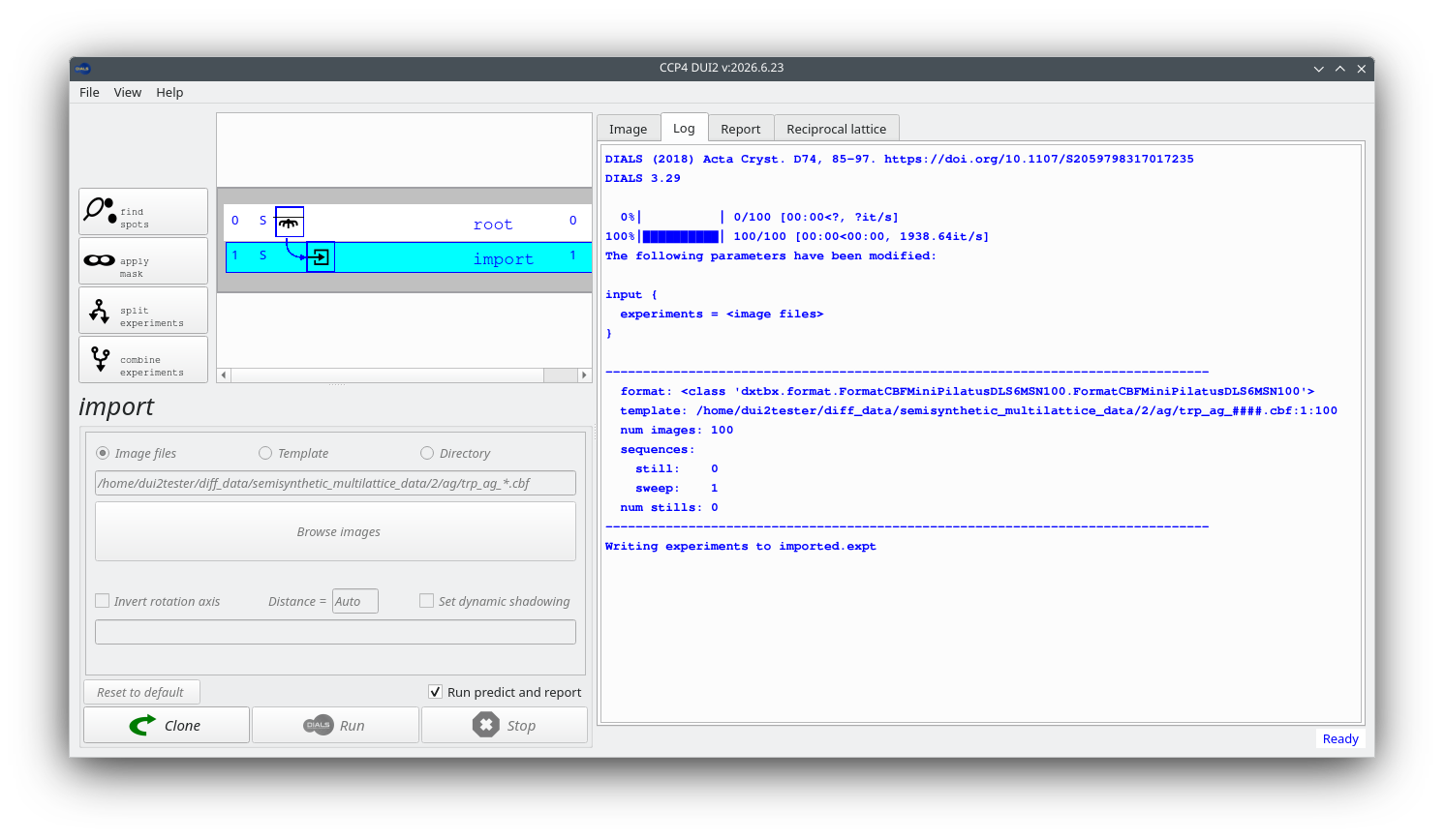
Select "find spots" from the left-hand panel. Under the "Advanced" tab of the parameter area, use the search box at the top of the parameter list to find and set:

• min_spot_size → 3

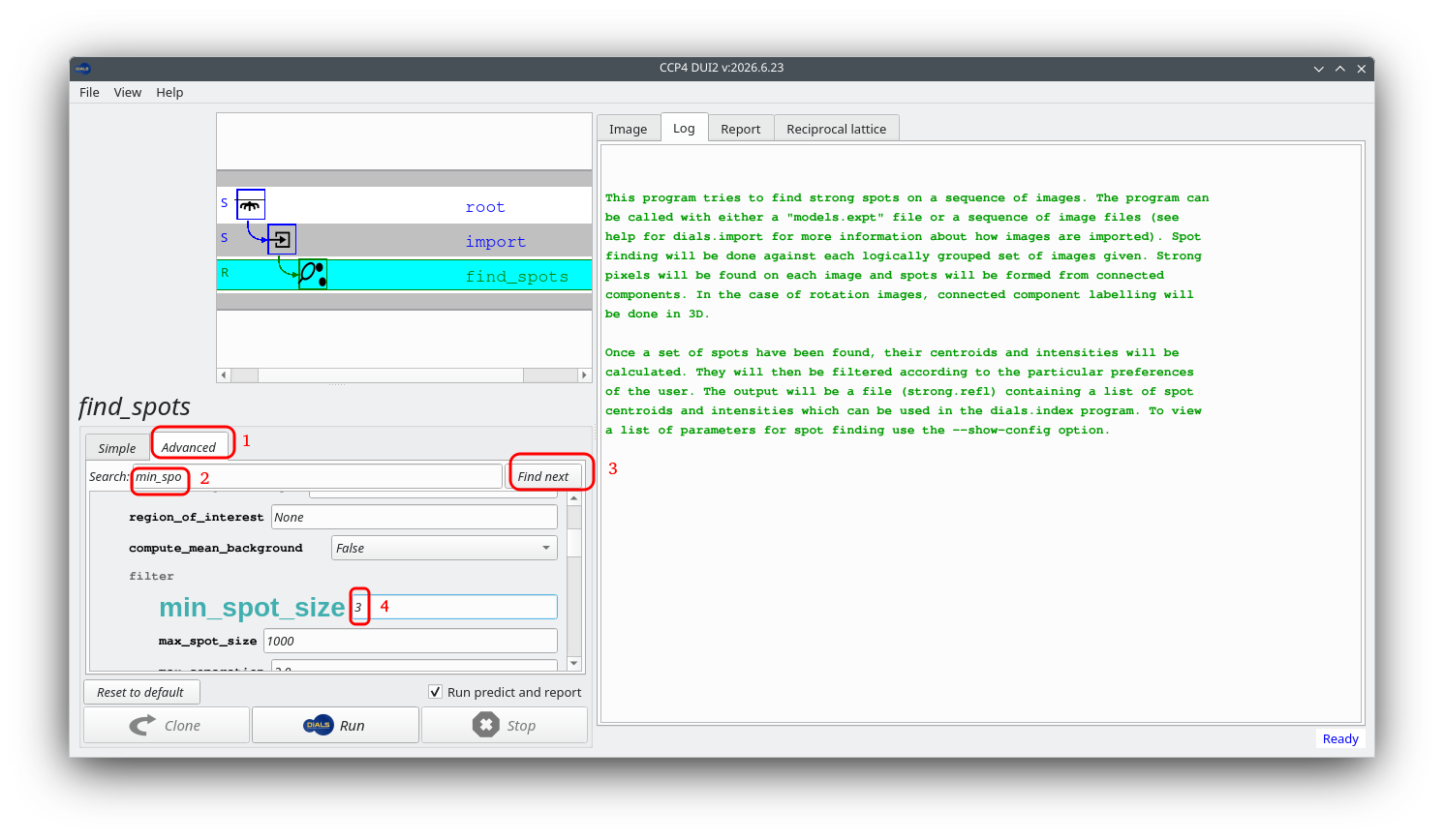
This removes very small pixel islands that are not genuine Bragg spots. Click Run. The log reports a large number of spots found across 100 images.

3. Index — single lattice first

Select "index" from the left-hand panel and click Run with default parameters.

Inspect: the evidence for a second lattice shows up clearly across all four visualisation tabs:

• "Image" tab — toggle between observed and predicted reflections. Predictions match well for one orientation, but a systematic set of strong spots remains unpredicted throughout the scan.
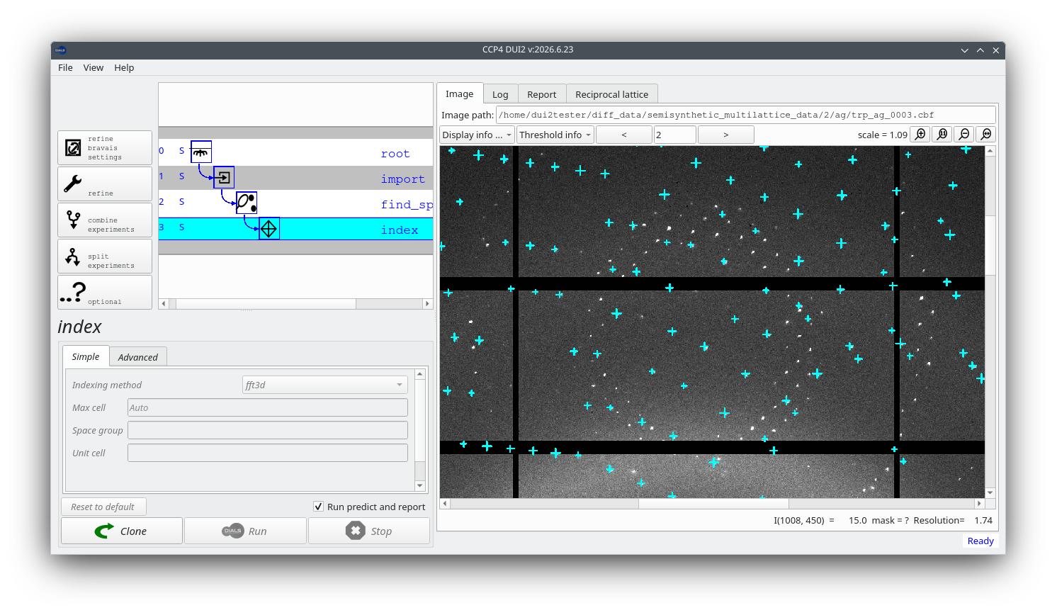
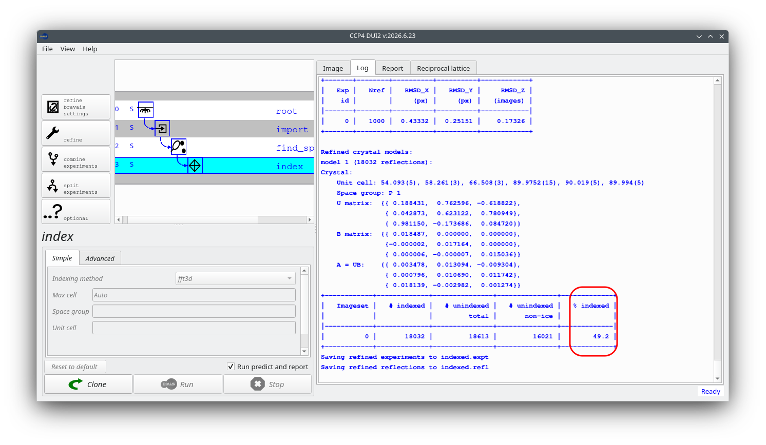
• "Log" tab — the fraction of indexed spots will be noticeably lower than the 80–95% expected for a clean single-lattice dataset.
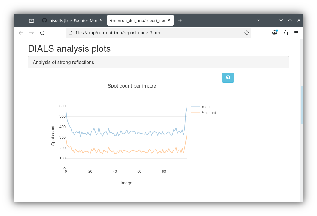
• "Report" tab — in the "Analysis of strong reflections" section, look at the "Spot count per image" graph. Only around half the found spots appear as indexed — a clear sign that a significant population has been left out.

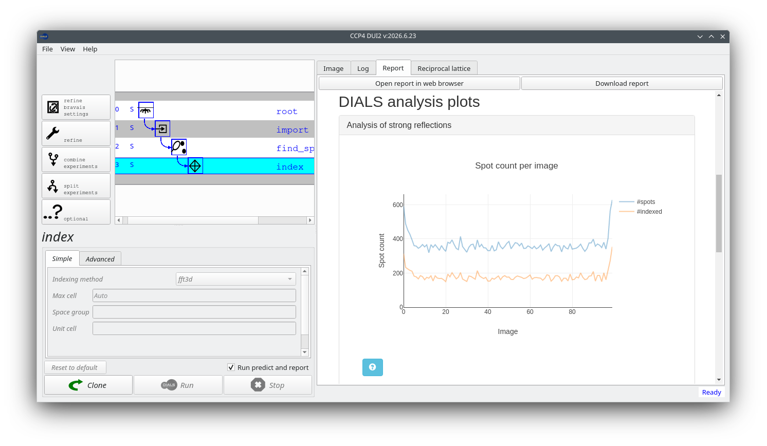
the report may not render automatically inside the app — if that happens, click "Open report in web browser" to view it.

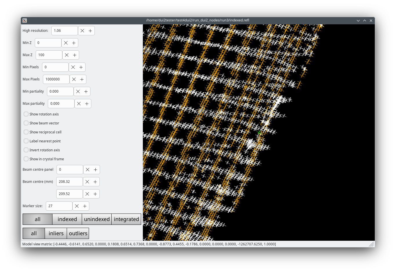
• "Reciprocal lattice" tab — open the viewer. Indexed spots are shown in one colour, unindexed in another. Rather than a random scatter, the unindexed spots form their own ordered rows in reciprocal space — the unmistakable signature of a second lattice.

4. Clone and re-index with two lattices

Make sure the index node from step 3 is selected in the history tree, then click "Clone" in the bottom-left corner of the GUI, below the parameter area. This creates a new independent copy of the index node, branching from the same find-spots input, with the same parameters ready to edit. The original single-lattice node is preserved as a reference in the history tree.

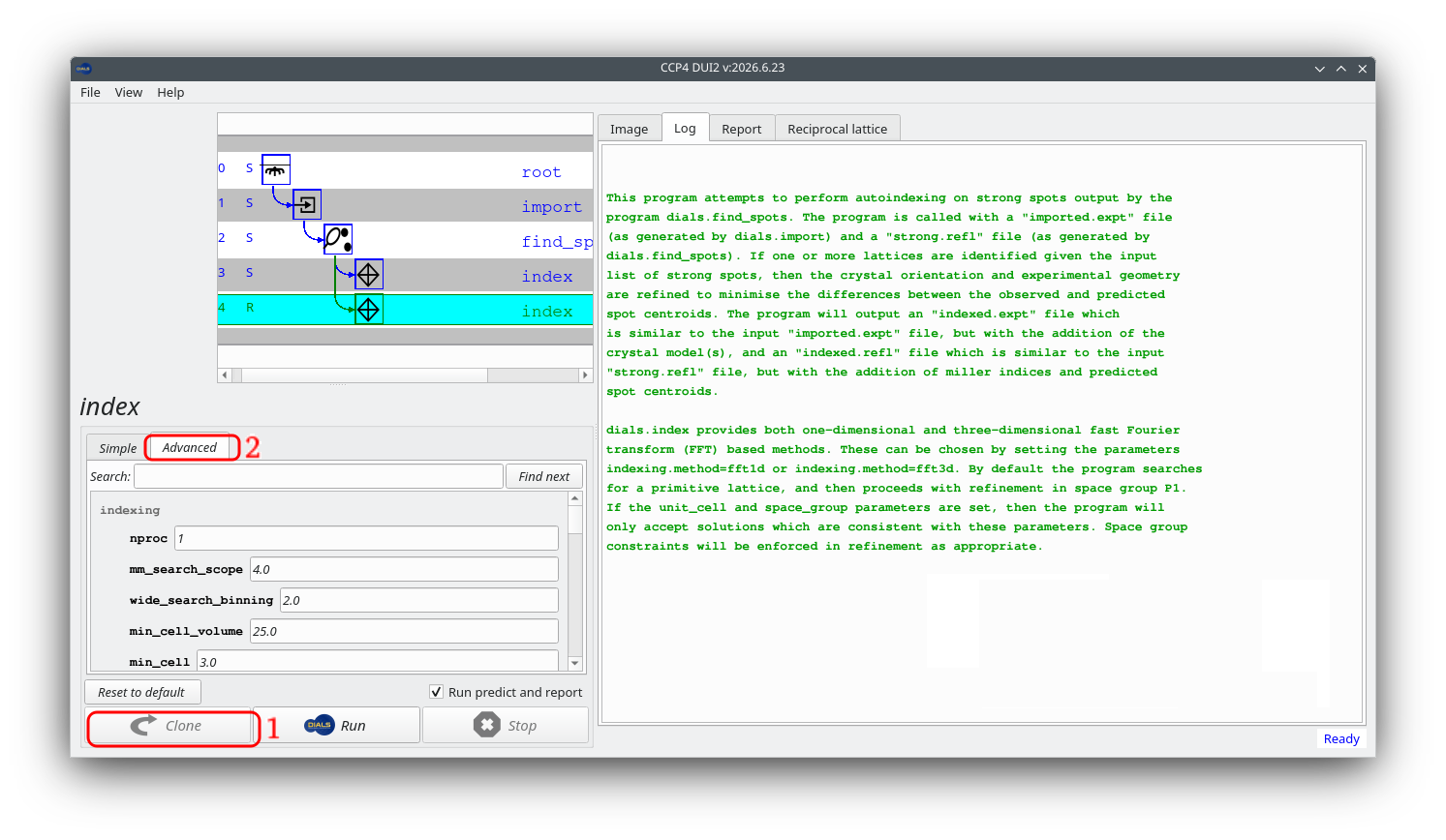
In the parameter area of the cloned node, under the "Advanced" tab, use the search box again to find and set:

• max_lattices → 5

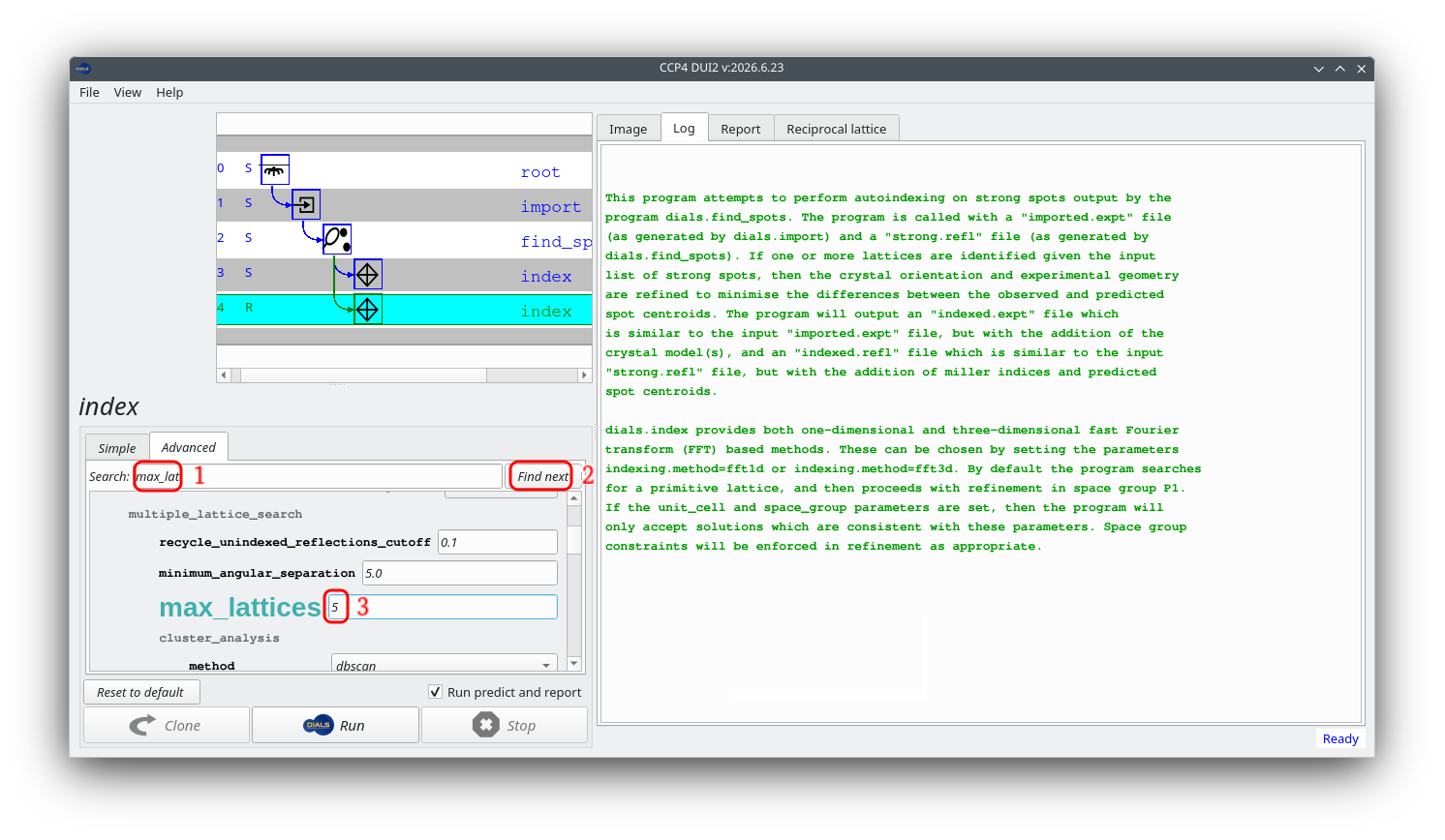
Setting this higher than the number of lattices you expect is a safe approach — DIALS will search for up to five lattices but stop as soon as there are not enough unindexed spots left to justify finding another one. For this dataset it will find exactly two. Click Run. The log reports two refined crystal models, together accounting for roughly 95% of all strong spots.

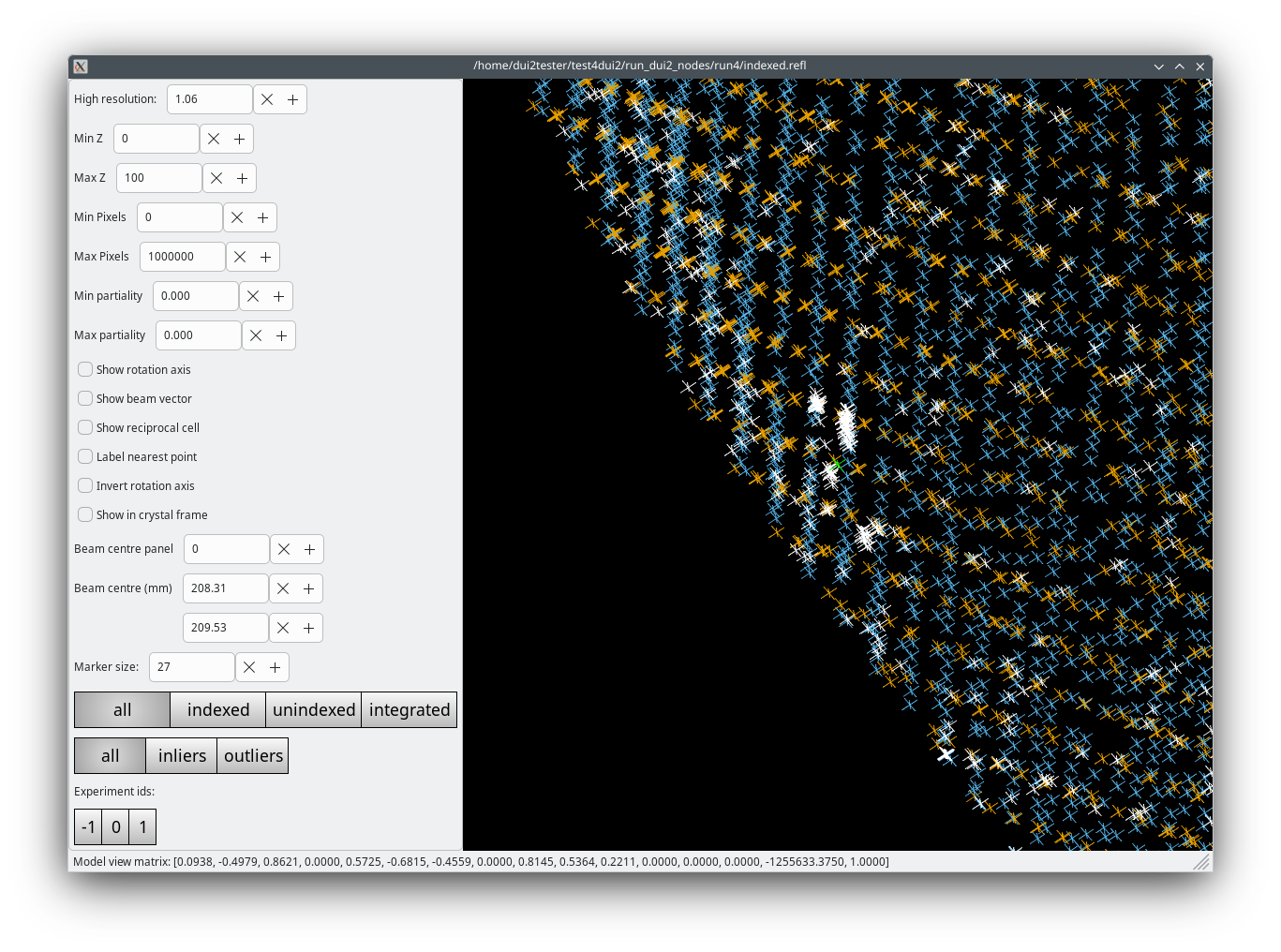
Inspect: reopen the reciprocal lattice viewer. Spots are now coloured by lattice assignment — two clearly distinct orientation families, each forming clean rows, with very few unindexed spots remaining.

5. Split experiments

Select "split experiments" from the left-hand panel and click Run. DUI2 splits the two crystal models into two independent child nodes in the history tree — one for each lattice. From this point forward, each branch is processed exactly like a standard single-lattice dataset.

Inspect: click on the first branch node in the history tree, then open the "Image" tab. Only the reflections belonging to lattice 0 are shown — predictions and observations for lattice 1 are hidden. Click on the second branch node and the display switches to lattice 1 only.

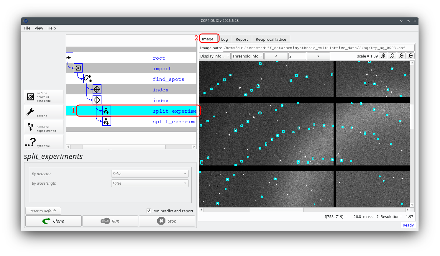
Scroll through several images on each branch. Do the predicted positions match the observed spots well on both branches? This is the moment to make a practical decision: if one lattice shows a poor fit between model and experiment throughout the scan, there is no obligation to process it further. You can simply continue with the better branch alone — this is equivalent to selecting the crystal that diffracted well and discarding the one that did not.

For this dataset both lattices should look good. Continue with both branches.

---

Chapter 2: Process

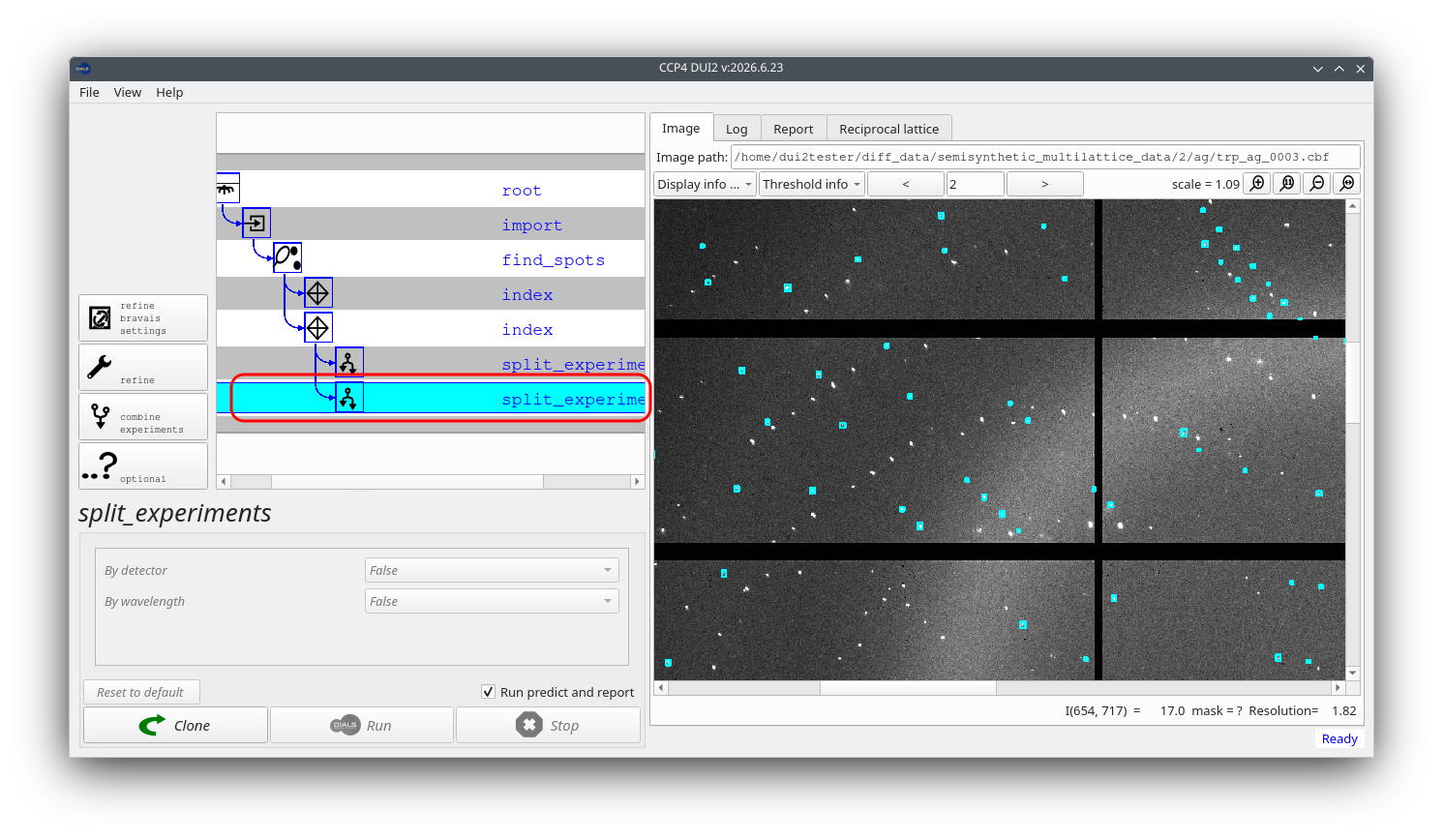
From this point, the two branches are independent. The steps below are identical for both, and the order in which you process the two branches does not matter — work through them on one branch first, then repeat on the other. The instructions refer to a single branch for clarity.

6. Refine Bravais settings

With a branch node selected in the history tree, select "refine bravais settings" from the left-hand panel and click Run. A table of candidate Bravais lattice solutions is written to the log.

7. Reindex

Select "reindex" from the left-hand panel. DUI2 displays an interactive table of the solutions from the previous step. Click the row corresponding to solution 5 — primitive orthorhombic (oP, P 2 2 2) — and DUI2 runs dials.reindex automatically with that choice.

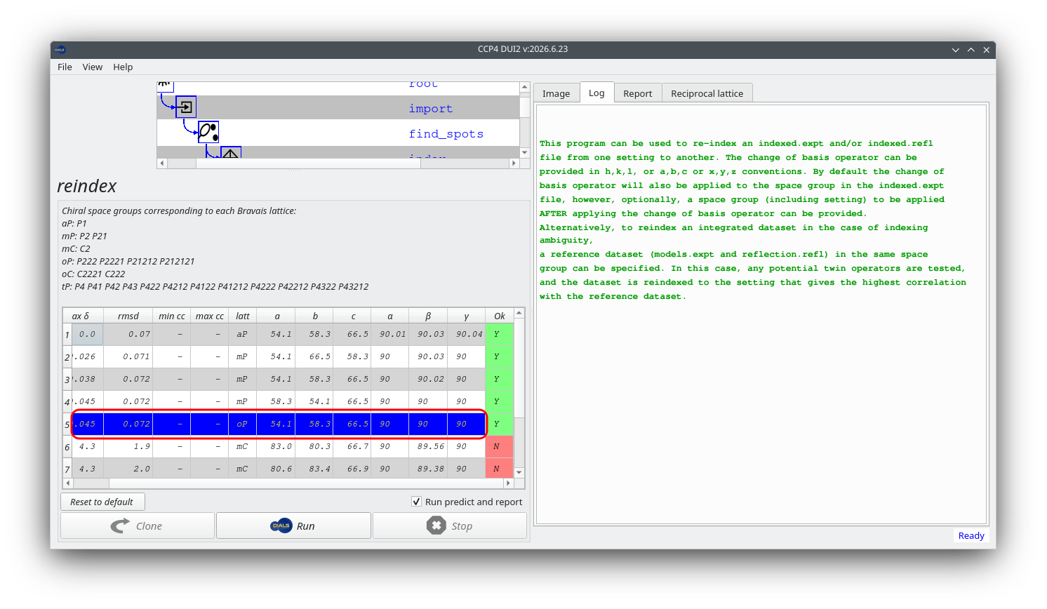
The chosen solution should have a metric fit significantly closer to zero than the other solutions, and be marked acceptable. If the highest-symmetry acceptable solution differs between the two branches, that is a signal worth investigating before continuing.

8. Refine

Select "refine" from the left-hand panel. Under the "Simple" tab, set:

• Outlier rejection algorithm → tukey

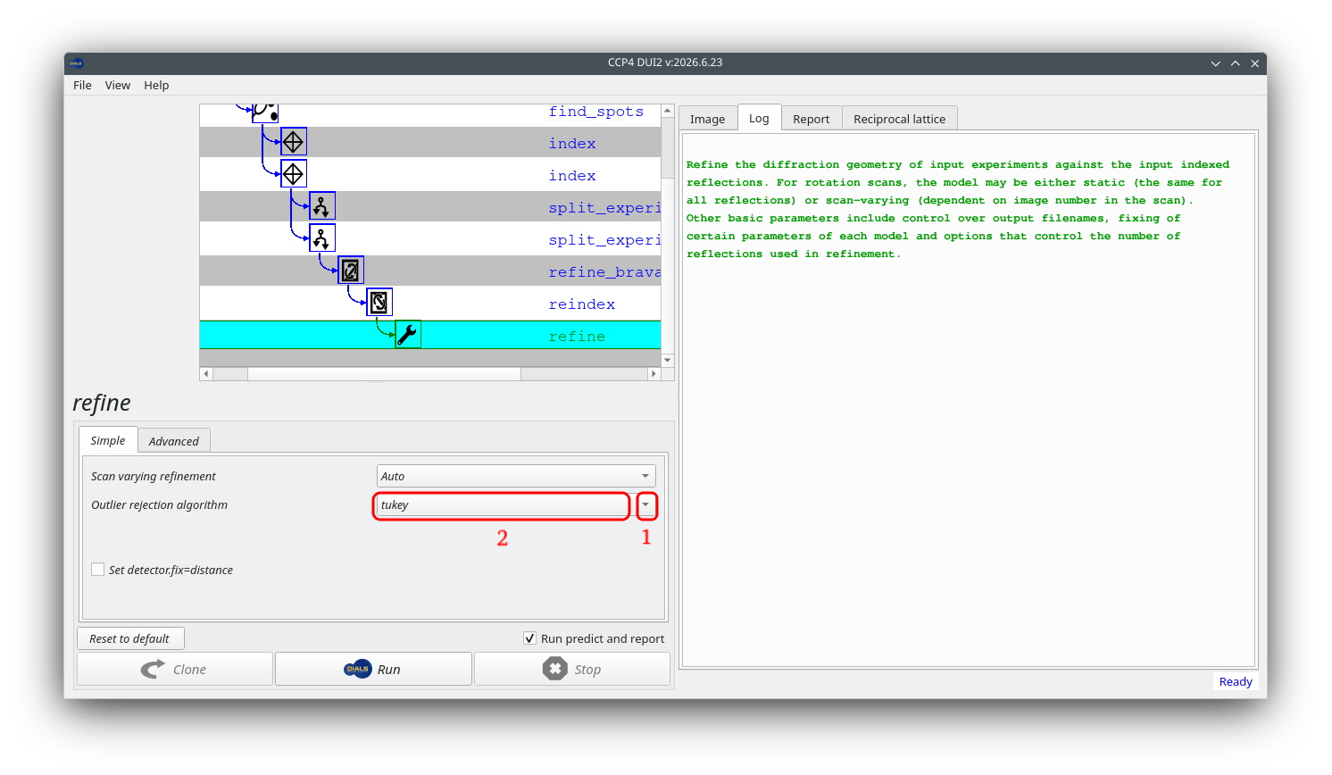
Click Run. Scan-static and scan-varying refinement runs for this lattice. Check the "Report" tab — changes in cell parameters and orientation angles across the scan should look small and smooth.

9. Integrate

Select "integrate" and click Run with default parameters. Check the end of the log for the "Summary for experiment 0" section — I/σ(I) and cc_prf should look reasonable.

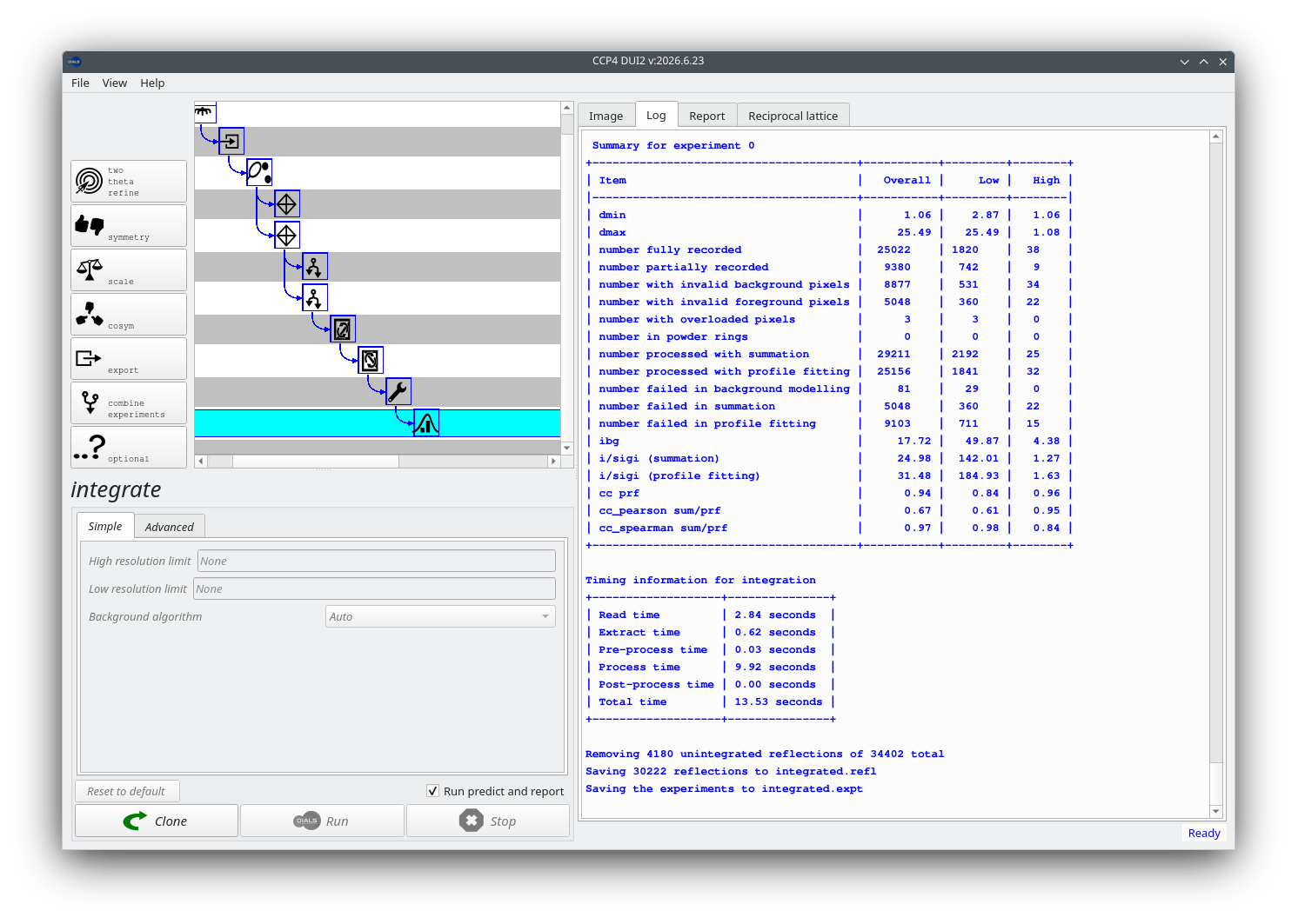
Once steps 6–9 are complete on branch 1, go back to the split experiments node in the history tree, select branch 0, and repeat steps 6–9 for this lattice.

---

Chapter 3: Post integration

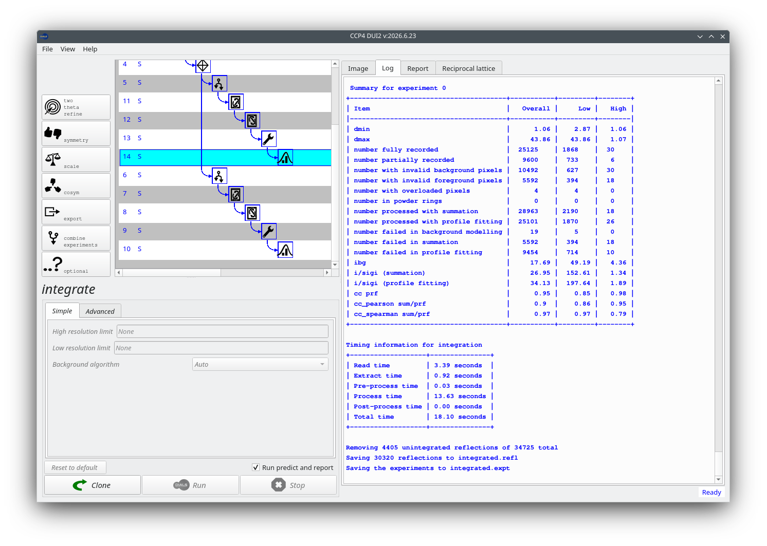
With both branches refined and integrated, the remaining steps — symmetry determination, scaling, and export — can be run independently on each branch. Run the following steps on each branch in turn.

10. Determine crystal symmetry

Select "symmetry" and click Run. The analysis should return P m m m as the Laue group, with clear 2₁ screw axes indicating an orthorhombic space group. If you are using the first dataset, the result should be P 2 2₁ 2₁ — if you chose a different dataset from the archive, the specific assignment of screw axes to unit cell axes may differ (e.g. P 2₁ 2 2 or P 2 2₁ 2), which is simply a matter of axis labelling convention rather than a different crystal form.

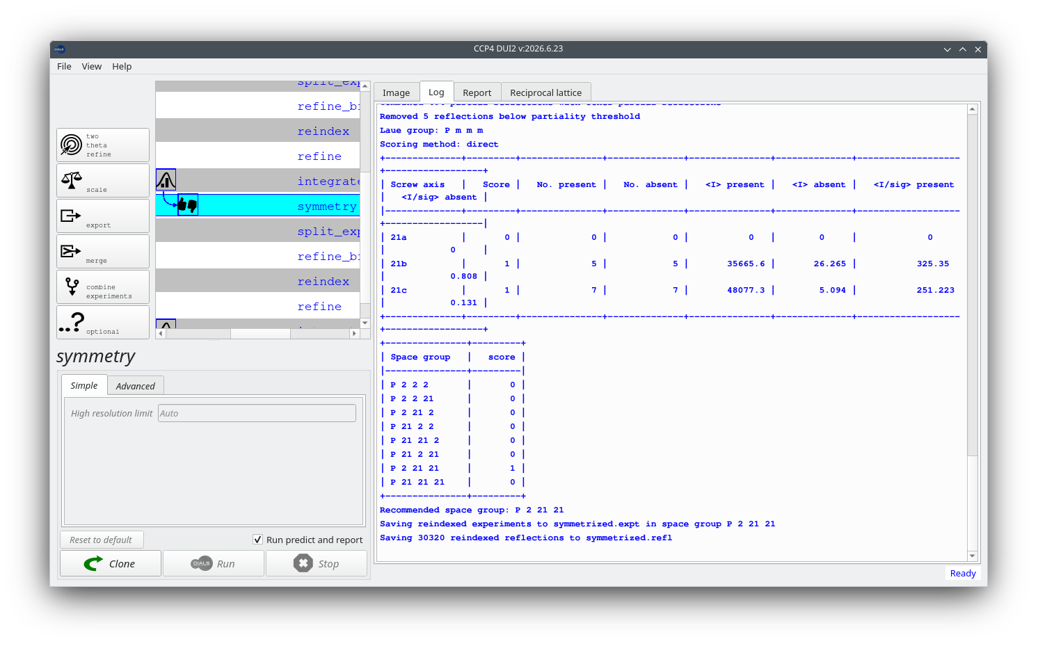
No reflections are available to test the 2₁ screw along a for this dataset — it is worth testing both P 2 2₁ 2₁ and P 2₁ 2₁ 2₁ during structure solution.

11. Scale

Select "scale" and click Run with default parameters. Check the "Report" tab for resolution-dependent statistics.

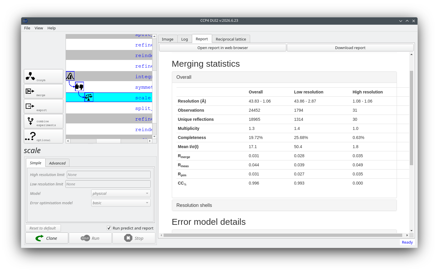
The data has not yet been merged at this stage — dials.scale reports merging statistics but retains all observations.

12. Export

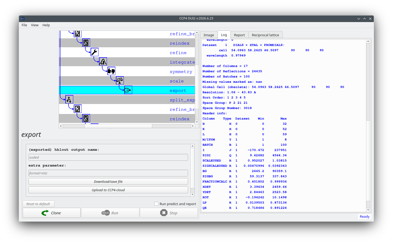
Select "export" and click Run, then "Download/save file" to write the MTZ file for this lattice to your processing directory. Repeat on the second branch to obtain a separate MTZ for each lattice.

To upload directly to CCP4 Cloud: in Cloud, note your project ID and copy the "CloudRun Id" from the "My Account" page. Back in DUI2, press "Upload to CCP4-cloud" and fill in the dialog. This creates a cloudrun node that imports the MTZ into your Cloud project. Repeat for the second branch if you want both lattices available in Cloud.

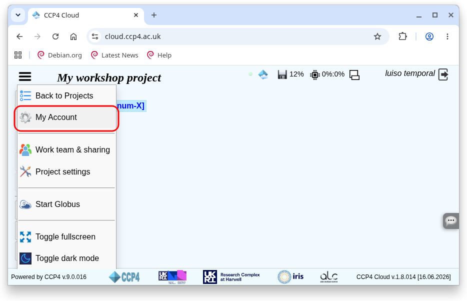
To upload from to CCP4 Cloud: in Cloud, follow the next steps:

Uploading manually (no cloudrun available)

Not every DUI2 installation has access to a local CCP4/cloudrun environment — if you installed DUI2 standalone, the "Upload to CCP4-cloud" button above will fail or be unavailable, since it depends on a cloudrun subprocess. In that case, upload the exported MTZ file directly through the CCP4 Cloud website instead:

1. In CCP4 Cloud, open your project's task list and click "File(s) Upload and Import" to create a new upload task.

   

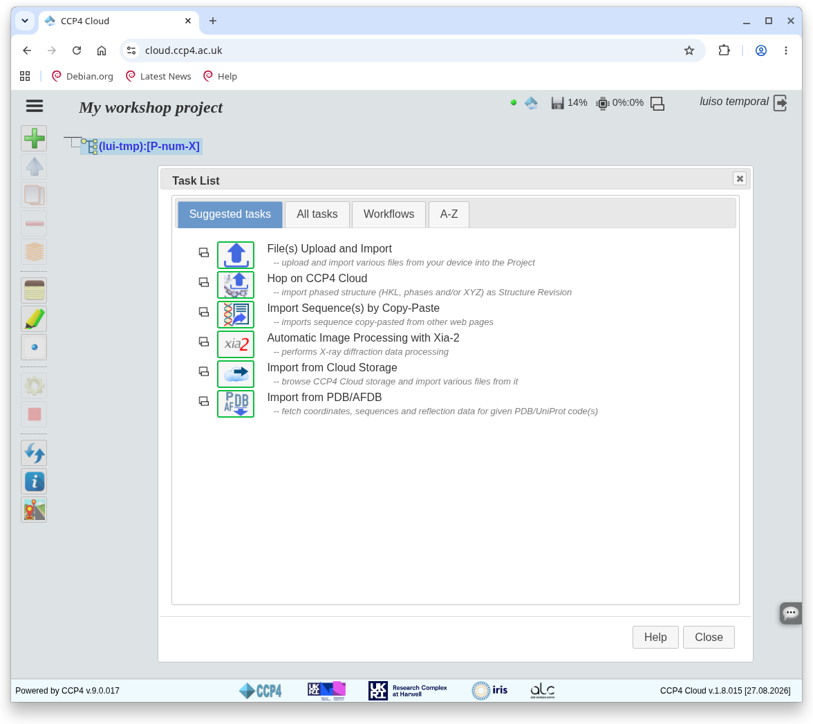
2. The task opens a "File import (new)" dialog. Click "Upload file(s)".

   

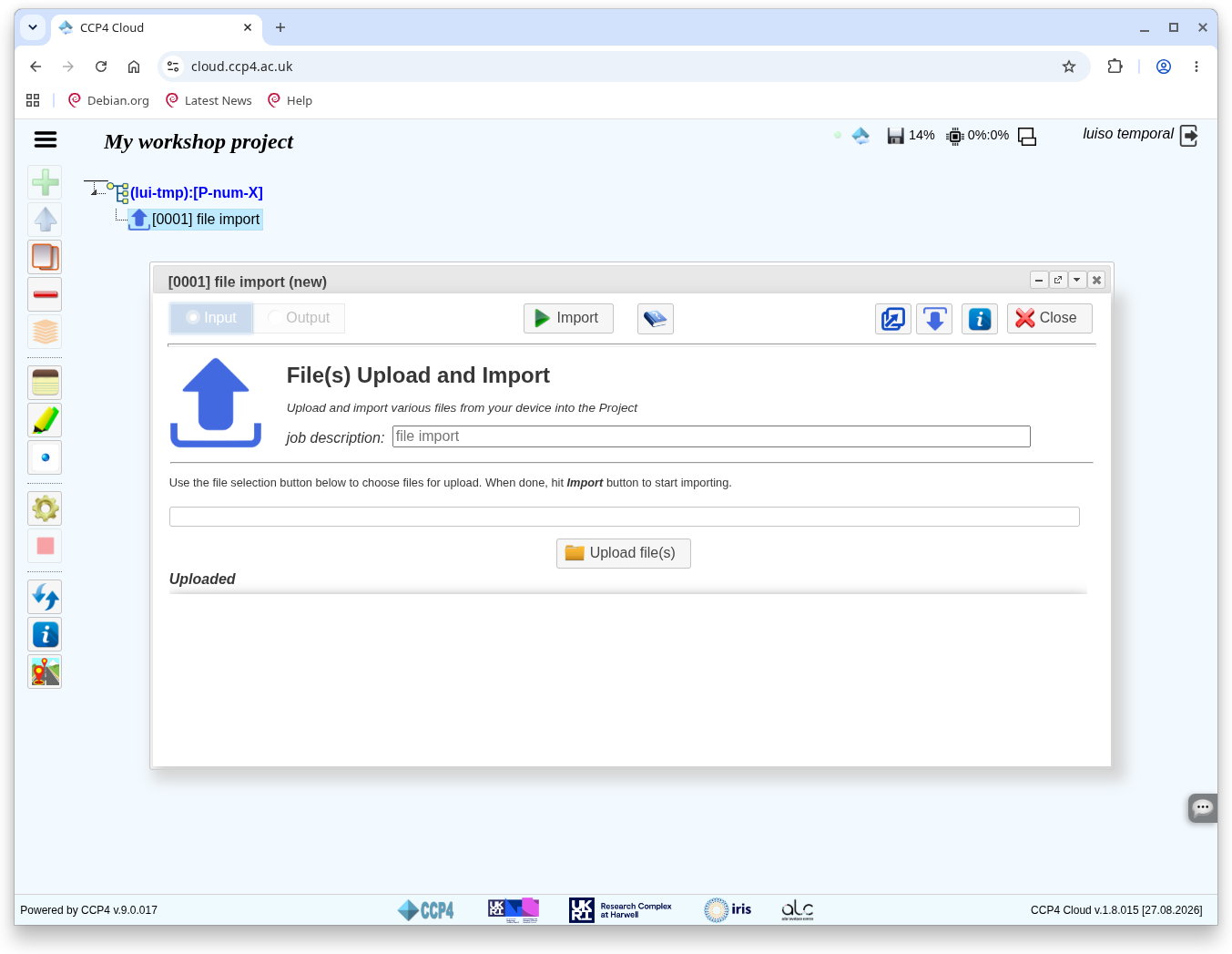
3. Choose the MTZ file from step 12 in your computer's file browser. Once it uploads, a new dialog appears on top of the previous one — click "Close".

   

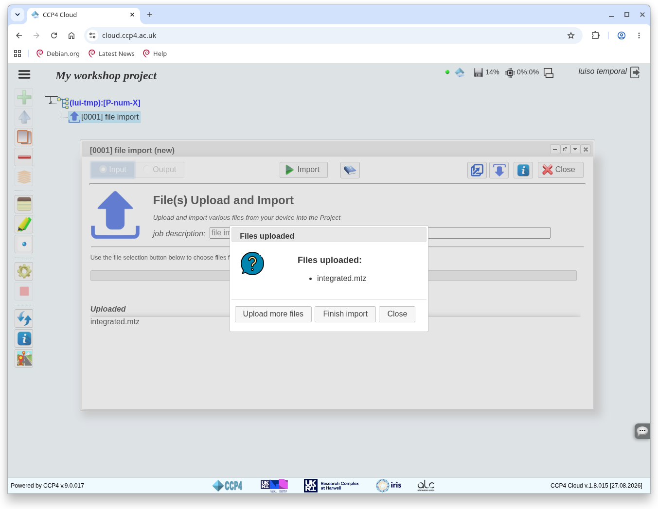
4. The "File import" dialog now reads "completed" and lists the uploaded file in a table — your MTZ is now in the CCP4 Cloud project.

   

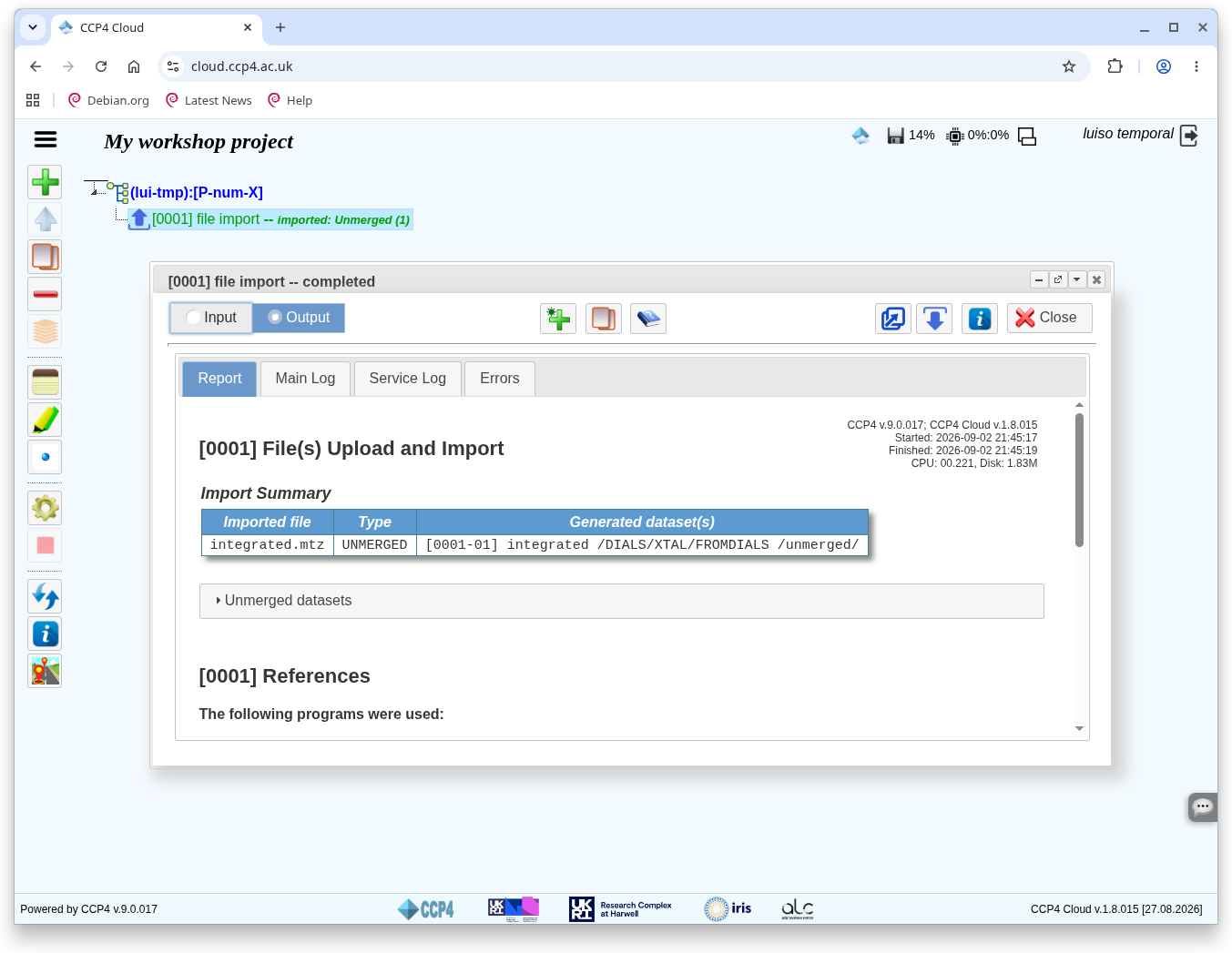
Repeat this on the second branch's exported MTZ if you want both lattices available in Cloud.