All About Graphs (not really!)
A guide to Kronecker graphs and the technical implementation in this project.
Kronecker graphs are synthetic graphs designed to resemble social network graphs.
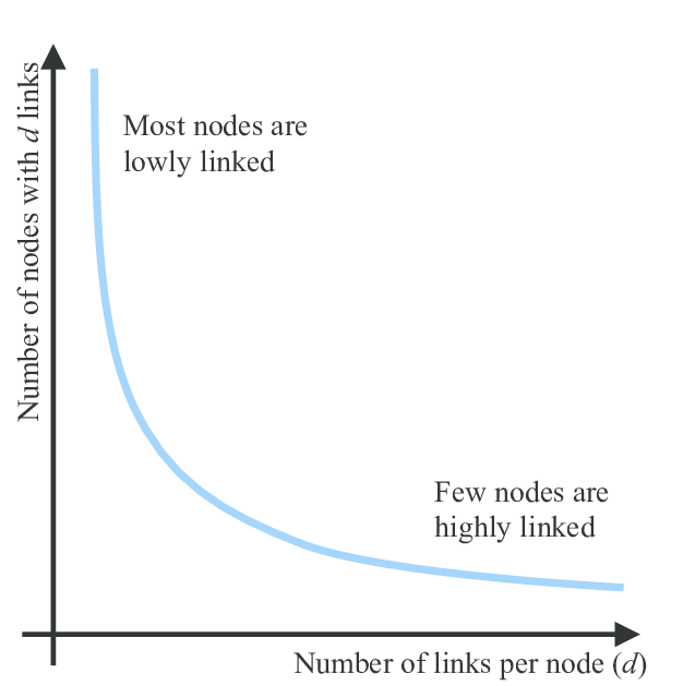
These graphs are characterized by the power law distribution. That means there are a lot of nodes with very low degrees and few nodes with very high degrees. The above image demonstrates this (note it's in log scale). Imagine the number of Twitter followers a celebrity like Obama has compared to Chris (none in this case:)).
To generate Kronecker graphs, we are piggybacking off of Scott Beamer's GAP Benchmark Suite which uses a R-MAT generator with the parameters supplied by the Graph500 specification. We only care about two things, the scale of the graph scale and the average degree edgefactor. Our generated graph will have 2^{scale} number of nodes and 2^{scale} * edgefactor number of edges.
The graph generator could be found under util/graphgen. Modify util/graphgen/graphgen.cpp to generated a serial graph .sg and/or a weighted serial graph .wsg by toggling the UNWEIGHTED_ON and WEIGHTED_ON definitions respectively.
To compile the utility, run make. To generate the unweighted and/or weighted graphs, run ./graphgen.exe -g <scale> -k <edgefactor> (note for Graph500, edgefactor=16). Optionally, remove the utility with make clean.
A graph consists of nodes and neighbors. The graphs typically represented in Compressed Sparse Row (CSR) format, a sparse-matrix format. There's two arrays, the index array and the neighbors array. The index array indicates a particular node's neighbors should be accessed. The neighbors array contains the neighbor node id and other relevant information (e.g., edge weight).
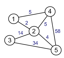
In this example, the index and neighbors array look like this. Notice how the size of the index array is # nodes + 1. Since the nodes in this graph are 1-indexed, we relabeled them to be 0-indexed (e.g., node 1 in the graph is node 0). For a node u, it's neighbors in the neighbors array span from index[u] to index[u + 1] (exclusive).
index     = [0, 2, 6, 8, 11, 14]
neighbors = [1, 3, 0, 2, 3, 4, 1, 4, 0, 1, 4, 1, 2, 3] // 0-indexed labeling.
Example Usage: To get the neighbors of node 2 (as represented by the graph above), we need to iterate from index[1] to index[1 + 1] = index[2] (note that we convert 1-indexed node labels to 0-index node labels).
nid_t u = 1; // NOde 2 in 0-indexed format.
for (nid_t i = index[1]; i < index[1 + 1]; i++)
    nid_t v = neighbors[i]
    print "Edge from node " + u + " to node " + v "."

// Expected output:
// Edge from node 1 to node 0.
// Edge from node 1 to node 2.
// Edge from node 1 to node 3.
// Edge from node 1 to node 4.
Visually, we can see which elements of the neighbors array is accessed.
neighbors = [2, 4, 1, 3, 4, 5, 2, 5, 1, 2, 5, 2, 3, 4]
                   ^  ~  ~  ~  ^
                index[1]    index[2] (exclusive)
Likewise, for a weighted graph, the index array would be the same but the neighbors array may look something like this (where each tuple is (neighbor node id, edge weight)).
neighbors = [(1, 2), (3, 5), (0, 2), (2, 14), (3, 5), (4, 4), (1, 14), ... , (3, 58)] // 0-indexed labeling.
Example Usage: To get the neighbors and edge weights of node 2 (as represented by the graph above), we can perform a similar operation.
nid_t u = 1; // Node 2 in 0-indexed format.
for (nid_t i = index[u]; i < index[u + 1]; i++)
    nid_t    v = neighbors[i][0] // First element of tuple.
    weight_t w = neighbors[i][1] // Second element of tuple.
    print "Edge from node " + u + " to node " + v + " has a weight of " + w + "."

// Expected output:
// Edge from node 1 to node 0 has a weight of 2.
// Edge from node 1 to node 2 has a weight of 14.
// Edge from node 1 to node 3 has a weight of 5.
// Edge from node 1 to node 4 has a weight of 4.
Visually, we can see which elements of the neighbors array is accessed.
neighbors = [(1, 2), (3, 5), (0, 2), (2, 14), (3, 5), (4, 4), (1, 14), ... , (3, 58)] // 0-index labeling.
                             ^~~~~~  ~~~~~~~  ~~~~~~  ~~~~~~  ^
                          index[1]                         index[2] (exclusive)
The index array for serial graphs is represented by offset_t and the neighbors array is represented by nid_t. To serialize this graph, perform this.
// file is opened in binary mode.
write(# of nodes, sizeof(nid_t))
write(len(neighbors array), sizeof(offset_t))
write(index array, (# of nodes + 1) * sizeof(offset_t))
write(neighbors array, len(neighbors array) * sizeof(nid_t))
A C++ implementation could be found in src/gapbs/gapbs.cuh under std::ostream &operator<<(std::ostream &os, const GapbsGraph g).
Weighted serial graphs are very similar to serial graphs. The index array for serial graphs is represented by offset_t and the neighbors array is represented by wnode_t. To serialize this graph, perform this.
// file is opened in binary mode.
write(# of nodes, sizeof(nid_t))
write(len(neighbors array), sizeof(offset_t))
write(index array, (# of nodes + 1) * sizeof(offset_t))
write(neighbors array, len(neighbors array) * sizeof(wnode_t))
A C++ implementation could be found in src/gapbs/gapbs.cuh under std::ostream &operator<<(std::ostream &os, const GapbsWGraph g).
More graphs could be found listed under the KONECT project by Jérôme Kunegis