Spatial tessellation, modeling, and cross-validation toolkit for R


spatialkit is a modular R package for end-to-end spatial analysis workflows built on sf: CRS management, Voronoi/Delaunay/grid tessellation, feature-to-polygon assignment and aggregation, geographically weighted regression (GWR via GWmodel), Bayesian spatial Gaussian-process regression (via brms), and — the part most spatial ML pipelines get wrong — spatially aware cross-validation with block and buffered leave-one-out strategies that respect the autocorrelation structure of the data.
All model backends return a common spatial_fit S3 object with consistent predict(), fitted(), residuals(), coef(), and summary() methods, so models can be fitted, cross-validated, and compared through one interface.
The idea in three steps:
- Cut geography into cells. Grow Voronoi regions from k-means seeds, lay down hex or square grids, or triangulate — clipped to your study area, with stable reproducible cell IDs.
- Model what varies across space. Fit geographically weighted regression or a Bayesian Gaussian process through one common interface, and aggregate observations per cell with honest, autocorrelation-aware standard errors.
- Validate without fooling yourself. Build cross-validation folds that hold out whole regions sized to the data's autocorrelation range, instead of leaking spatial signal between train and test.
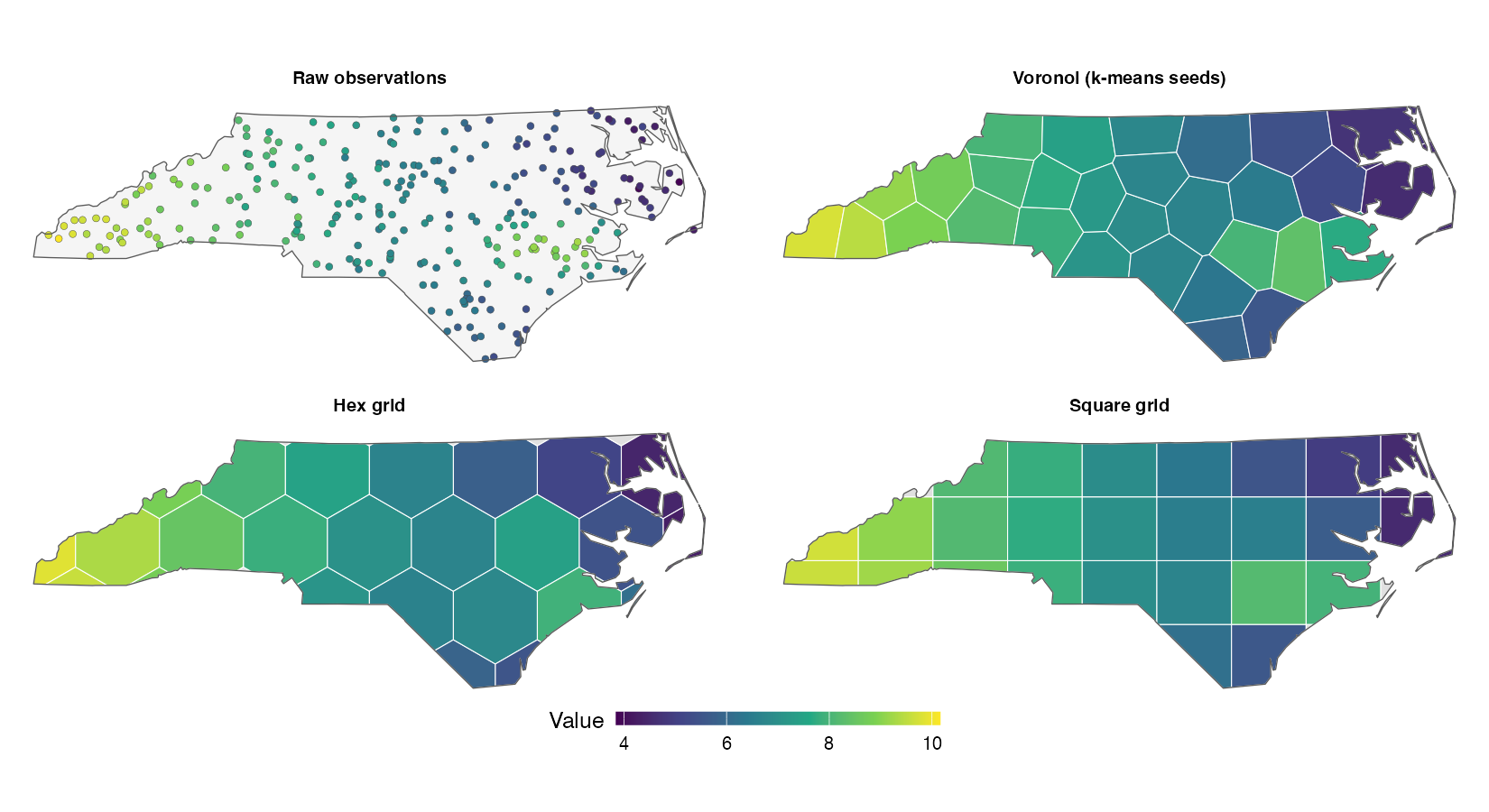
Three ways to cut the same geography. The first panel shows raw observations of a smooth spatial field over North Carolina (high in the west, with an eastern hotspot). The other panels show the same points aggregated into Voronoi regions grown from k-means seeds, a hex grid, and a square grid — each cell coloured by the mean of the points that fall inside it (computed with assign_features_to_polygons() + summarize_by_cell()). All panels share one colour scale, so each tessellation should look like a mosaic version of the raw data:
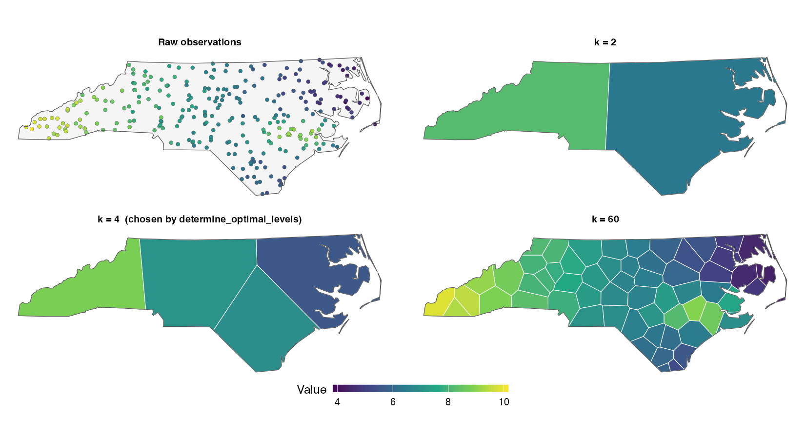
Resolution is a modeling decision, not a cosmetic one: too few cells smooth the signal away, too many leave each cell with a handful of noisy observations. determine_optimal_levels() chooses candidate cell counts for you by combining two criteria — a geometric elbow on the within-cluster sum of squares from a k-means sweep, and a model-aware check that computes Moran's I on OLS residuals at each candidate resolution. The Moran's I profile measures how much spatial structure in the response remains unexplained at that scale, so the combined ranking picks the resolution that balances parsimony against residual spatial independence:
k <- determine_optimal_levels(pts, response_var = "price",
                              predictor_vars = "elev", max_levels = 15)
The same field cut at three resolutions, next to the raw observations — too coarse blurs the hotspot, too fine chases noise with near-empty cells, and the selected k preserves the trend without overfitting geography:
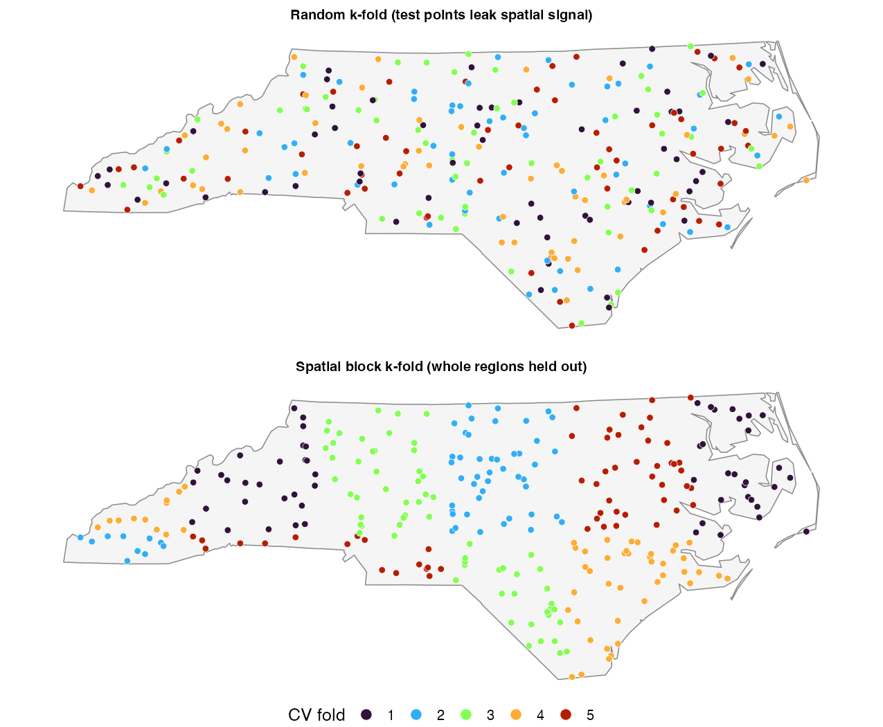
Random k-fold CV leaks information between spatially correlated train and test observations, producing optimistic performance estimates. spatialkit builds folds from spatial blocks sized to the data's autocorrelation range (estimated from directional variograms via estimate_sac_range()), or from distance-buffered leave-one-out splits, so that reported metrics reflect true out-of-sample spatial generalization.
The difference is easy to see. On the same North Carolina sites, random folds scatter test points among their spatially correlated training neighbours, while block folds hold out contiguous regions:
# From GitHub
# install.packages("remotes")
remotes::install_github("elkronos/gis_modeling_toolkit")

# From a local clone
devtools::install("path/to/spatialkit")
Hard dependencies (sf, dplyr, logger, digest) install automatically. Optional backends are declared in Suggests and checked at runtime:
| Feature | Requires |
|---|---|
| GWR modeling | GWmodel, sp |
| Bayesian GP modeling | brms (with rstan, or the non-CRAN cmdstanr backend if installed) |
| Delaunay triangulation | geometry |
| Variogram-based autocorrelation range | gstat |
| PSIS-LOO information criterion | loo |
| Plotting | ggplot2 |
| Fast k-NN weights (recommended for n > 5,000) | FNN, Matrix |
A self-contained example with synthetic data:
library(spatialkit)
library(sf)

# --- Synthetic point data in a projected CRS -------------------------------
set.seed(1)
n  <- 200
df <- data.frame(x = runif(n, 0, 5000), y = runif(n, 0, 5000))
df$elev  <- rnorm(n)
df$price <- 50 + 0.004 * df$x + 3 * df$elev + rnorm(n)
pts <- st_as_sf(df, coords = c("x", "y"), crs = 32632)

# --- Tessellate the study area ---------------------------------------------
tess <- build_tessellation(pts, method = "voronoi")
plot_tessellation_map(tess$cells, features_sf = pts)

# --- Aggregate observations per cell ---------------------------------------
assigned <- assign_features_to_polygons(pts, tess$cells, polygon_id_col = "cell_id")
cells    <- summarize_by_cell(assigned, response_var = "price",
                              predictor_vars = "elev", deff = "kish")

# --- Spatially blocked cross-validation folds ------------------------------
folds <- make_folds(pts, k = 5, method = "block_kfold",
                    auto_range = TRUE, response_var = "price",
                    predictor_vars = "elev", seed = 42)

# --- Fit and cross-validate a GWR model ------------------------------------
fit <- fit_gwr_model(pts, response_var = "price", predictor_vars = "elev")
cv  <- cv_gwr(pts, "price", "elev", folds = folds)
cv$overall        # pooled out-of-sample RMSE, MAE, R2, ...
cv$fold_metrics   # per-fold breakdown

# --- Residual spatial autocorrelation diagnostic ---------------------------
residual_morans_i(fit)
Compare backends head-to-head (each is fitted and cross-validated on identical folds):
comparison <- compare_models_cv(pts, "price", "elev",
                                models = c("GWR", "Bayesian"), k = 5)
comparison$overall| Area | Key functions |
|---|---|
| CRS & geometry | ensure_projected(), harmonize_crs(), coerce_to_points(), prep_model_data() |
| Tessellation | build_tessellation(), create_voronoi_polygons(), create_grid_polygons(), create_grid_polygons_cached(), clip_target_for(), ensure_stable_poly_id() |
| Seeding & resolution | get_voronoi_seeds(), voronoi_seeds_kmeans(), voronoi_seeds_random(), determine_optimal_levels() |
| Assignment & aggregation | assign_features_to_polygons(), summarize_by_cell() |
| Modeling | fit_gwr_model(), fit_bayesian_spatial_model(), gp_lengthscale_bounds(); S3: predict(), fitted(), residuals(), coef(), summary(), model_metrics() |
| Cross-validation | make_folds(), estimate_sac_range(), cv_gwr(), cv_bayes(), cv_spatial() |
| Comparison & diagnostics | compare_models(), compare_models_cv(), evaluate_insample(), residual_morans_i() |
| Plotting | plot_tessellation_map() |
cv_spatial() is the extensibility point: pass any fit_fn(train_sf) that returns a spatial_fit object and it plugs into the same fold infrastructure, metrics, and comparison tooling.
Both backends support true out-of-sample prediction — newdata needs only the predictor columns and geometry, not the response:
new_sites <- st_sf(
  elev = c(0.5, -1.2),
  geometry = st_sfc(st_point(c(1000, 2000)), st_point(c(3000, 4000)), crs = 32632)
)
preds <- predict(fit, newdata = new_sites)
newdata is automatically transformed to the CRS used during fitting, rows with missing or non-finite predictors return NA (output length always matches nrow(newdata)), and non-point geometries are coerced to representative points. The Bayesian method additionally supports type = "predict" for full posterior predictive draws and draws = TRUE for the raw draw matrix.
model_metrics() does require the response in newdata, since it computes error metrics against observed values.
All three CV functions accept a parallel argument for fold-level parallelism via parallel::mclapply() (macOS/Linux; falls back to sequential on Windows with a message). This matters most for cv_bayes(), where every fold is a full MCMC run:
cv <- cv_bayes(pts, "price", "elev", k = 5, parallel = TRUE)  # auto-detect cores
cv <- cv_gwr(pts, "price", "elev", k = 5, parallel = 4L) # explicit countResidual Moran's I. residual_morans_i() computes Moran's I on model residuals with the Cliff & Ord randomisation variance, using row-standardised k-NN weights by default (sparse via FNN + Matrix when available) or a user-supplied weight matrix (base or sparse Matrix). compare_models() runs it automatically and warns when residual spatial structure remains.
Aggregation standard errors. The ..se_* columns from summarize_by_cell() are IID standard errors by default, which are anticonservative under within-cell spatial correlation. Pass deff = "kish" to apply Kish's design-effect correction from estimated intra-class correlations (separate ICCs for response and predictors), or a fixed numeric design effect. Inspect what was applied via attr(result, "deff_applied").
GWR collinearity. fit_gwr_model() checks the global condition number of the predictor matrix and spot-checks local condition numbers within bandwidth windows at sampled locations, since spatially clustered subsets can be collinear even when the global matrix is not.
GWR bandwidth fallback. If automatic bandwidth selection fails, a heuristic fallback is used, a warning() is raised, and fit$info$bandwidth_is_fallback = TRUE is set so downstream comparisons can flag the result. Supply an explicit bandwidth if you see this.
Bayesian GP anisotropy. fit_bayesian_spatial_model() standardizes X and Y coordinates independently before the GP term. This stabilises fitting but makes the kernel anisotropic in the original CRS whenever sd(X) ≠ sd(Y); the strategy is recorded in fit$info$coord_scaling$scaling_type. A data-informed GP length-scale prior is derived automatically from the inter-point distance distribution (see gp_lengthscale_bounds()).
Detailed diagnostics are logged to a session temp file, and warnings are echoed to the console. Logging is scoped to the "spatialkit" namespace and never touches your global logger configuration. To customize:
logger::log_appender(logger::appender_file("my_analysis.log"), namespace = "spatialkit")
logger::log_threshold(logger::WARN, namespace = "spatialkit")- Every exported function is documented: see
?fit_gwr_model,?make_folds, etc. - A worked end-to-end demo on the classic North Carolina dataset ships as a vignette (
vignettes/spatialkit_nc_demo.Rmd); build vignettes at install time withremotes::install_github(..., build_vignettes = TRUE), thenvignette("spatialkit_nc_demo"). - A runnable version of the demo is installed with the package:
system.file("scripts", "example_nc_demo.R", package = "spatialkit").
devtools::load_all()   # interactive development
devtools::test()       # run the test suite (~180 tests)
devtools::document()   # regenerate NAMESPACE + man/ from roxygen2
devtools::check()      # full R CMD check (vignette build requires pandoc)
The README figures are generated from actual package output; regenerate them with Rscript dev/make_readme_figures.R.
The test suite covers the core geometry/tessellation pipeline plus targeted regression tests for the statistical internals (Moran's I variance, CV fold/row-ID alignment, CRPS, hex-grid sizing, CRS alignment in prediction, and more). Tests that need optional backends (GWmodel, brms) skip automatically when those packages are not installed.
Contributions are welcome — please open an issue describing the bug or proposed change, and include a regression test with any fix.
MIT © Justin Chase. See LICENSE.
This is a personal project. It is not affiliated with, endorsed by, or connected to any organization. It uses public data sources only and was developed independently on personal time. No confidential, proprietary, or non-public information is included.