Reproducing Molecular Hydrogen VQE

Reproducing Molecular Hydrogen VQE

Reproduce the ideal VQE calculation behind P. J. J. O'Malley et al., “Scalable Quantum Simulation of Molecular Energies,” Physical Review X 6, 031007 (2016) using FlagQuantum. Follow each step as paper equation → derivation → corresponding code → numerical validation.

Paper: journal article and DOI. Numerical source: arXiv:1512.06860v2, revised February 4, 2017, PDF, Table I on PDF page 13. The authors explicitly identify v2 as correcting the identity coefficients in Table I. Use this corrected, pinned version throughout.

FlagQuantum version: 0.3.1, reference commit 5714b569cfc94e212b6d175eb7c87e1f36d8cf9d.

Verified: October 20, 2026, Python 3.12.14, PyTorch 2.13.0, NumPy 2.5.4, Matplotlib 3.11.2, macOS ARM64, CPU, float64 parameters and complex128 statevectors. All five complete Python files below were executed. No chemistry package, GPU, provider account, or QPU is required.

1. Define Exactly What Is Reproduced

Paper component	This tutorial	Evidence boundary
Eq. (1), Appendix A: reduced H2 Hamiltonian	All 54 corrected Table I rows, R=0.20 to 2.85 angstrom	Uses the paper's reduced STO-6G model; does not recompute orbital integrals or the fermion-to-qubit reduction.
Eq. (2): variational bound	Compare ansatz energies with dense eigenvalues	A small classical reference, not a scaling result.
Eq. (3): one-parameter UCC state	Implement the Pauli exponential with standard gates	Preserves logical wire labels and translates the displayed ket order.
Eq. (4), Fig. 2: weighted expectation surface	Scan 1000 angles in [-pi, pi), reusing five Pauli expectation curves	Exact noiseless simulator expectations replace superconducting-hardware measurements.
Fig. 3: molecular energy curve	Minimize each of the 54 tabulated geometry rows	Does not reproduce the original raw experimental data, readout correction, pulse errors, or fitted equilibrium geometry.
Classical feedback / gradients	Additional Adam loop and analytic gradient tests	A clearly marked differentiable extension; the experiment used an angle scan.
Finite measurement statistics	Separate three-basis shot experiment at R=0.75	Synthetic samples, not an experimental replication.

The paper's model is STO-6G, not the commonly substituted STO-3G tutorial model. Energy is in hartree (Eh) and bond length in angstrom. The corrected identity coefficient includes the geometry-dependent energy constant: do not add nuclear repulsion again. At R=0.75, the corrected constant is 0.2252; replacing it with -0.4804 changes every energy by -0.7056 Eh while leaving gradients unchanged. Correct gradients alone would miss this source-version error.

Start with From Papers and Equations to FlagQuantum Code, Qubit Ordering and Result Conventions, and Training Parameterized Circuits if these interfaces are unfamiliar.

2. Prepare and Run the Tutorial

Create a Python 3.12 environment, for example on macOS/Linux:

python3.12 -m venv .venv
source .venv/bin/activate
python -m pip install "flagquantum==0.3.1" "torch==2.13.0" "numpy==2.5.4" "matplotlib==3.11.2"
python -m pip check

See Installation and Compatibility for Windows activation and platform-specific PyTorch installation. The computations below explicitly use CPU.

Save the five complete files in one directory, or obtain the exact published files by cloning this Wiki:

git clone https://github.com/flagos-ai/FlagQuantum.wiki.git
cd FlagQuantum.wiki/examples/omalley2016
python h2_vqe_model.py
python verify_h2_vqe.py
python reproduce_h2_curve.py
python train_h2_vqe.py
python sample_h2_energy.py

The embedded coefficient table makes execution independent of PDF downloads or a live data service. reproduce_h2_curve.py creates vqe-results/ in the working directory, containing the CSV, environment manifest, and figure.

File	Purpose
h2_vqe_model.py	Pinned data, ansatz, expectation requests, analytical and dense references.
verify_h2_vqe.py	Check states, all five Pauli terms, energies, and four gradient routes.
reproduce_h2_curve.py	Run the 1000-angle scan at all 54 geometries and save the curve.
train_h2_vqe.py	Run an additional differentiable optimization at R=0.75.
sample_h2_energy.py	Estimate energy from independent Z/X/Y basis experiments and check its sampling error.

3. Paper Eq. (1): Translate the Hamiltonian and Data

Use Pauli labels to make coefficient order explicit:

$$H(R)=c_I I+c_{ZI}Z_0+c_{IZ}Z_1+c_{ZZ}Z_0Z_1+c_{XX}X_0X_1+c_{YY}Y_0Y_1.$$

This is the paper's Eq. (1) written with descriptive coefficient names. The main equation and Appendix A order XX/YY differently; the code reads the column labels, and both coefficients are equal in these data. At R=0.75:

Table I column	Value (Eh)	FlagQuantum request / code
Identity	0.2252	coefficients[0]; add classically, since its expectation is 1.
$Z_0$	0.3435	fq.expectation(fq.Z(0), name="zi")
$Z_1$	-0.4347	fq.expectation(fq.Z(1), name="iz")
$Z_0Z_1$	0.5716	fq.expectation(fq.Z(0) @ fq.Z(1), name="zz")
$X_0X_1$	0.0910	fq.expectation(fq.X(0) @ fq.X(1), name="xx")
$Y_0Y_1$	0.0910	fq.expectation(fq.Y(0) @ fq.Y(1), name="yy")

The complete 54-row CSV is embedded in h2_vqe_model.py and also available as h2-table.csv. The code checks its SHA-256, row count, geometry grid, and XX/YY equality. The transcribed fields are the first seven columns of Table I; the PEA timing, ordering, and Trotter-error columns are not inputs to VQE.

• PDF SHA-256: 79c6db488870611c9020adb2a6fc592a9d821f61266694567aa6c25cd54145c7
• CSV SHA-256: 1c2bed3d1cd1ef8cf266bf669501752fc5ddfa6f2f86fc19fa381b443b8af477

These checks identify the exact source/download and transcription used here. They do not turn rounded coefficients into higher-precision chemistry data.

4. Paper Eq. (3): Translate the State and Qubit Order

The paper writes $\lvert\varphi(\theta)\rangle=e^{-i\theta X_0Y_1}\lvert01\rangle$. Its Fig. 1 places q1 above q0, and Appendix B states that the Hartree-Fock input is prepared by flipping q0. FlagQuantum writes q0 as the most-significant bit. Keeping logical wire labels unchanged therefore gives:

Meaning	Paper's displayed ket	FlagQuantum ket / code
q0=0, q1=0	00	00
q0=1, q1=0: Hartree-Fock input	01	10; fq.Circuit(2).x(0)
q0=0, q1=1	10	01
q0=1, q1=1	11	11

Thus the same physical ansatz in FlagQuantum's vector order (00, 01, 10, 11) is

$$\lvert\psi(\theta)\rangle=e^{-i\theta X_0Y_1}\lvert10\rangle.$$

Do not prepare .x(1) merely to make the displayed string read 01. That would change the reference while keeping the coefficients fixed. At theta=0 and R=0.75, the correct HF energy is -1.124600000 Eh; the naive opposite input gives 0.431800000 Eh.

Derive the Amplitudes

Let $P=X_0Y_1$. Since $P^2=I$,

$$e^{-i\theta P}=\cos\theta\,I-i\sin\theta\,P,\qquad P\lvert10\rangle=i\lvert01\rangle.$$

Consequently,

$$\lvert\psi(\theta)\rangle= \cos\theta\lvert10\rangle+\sin\theta\lvert01\rangle =\begin{pmatrix}0\\\sin\theta\\\cos\theta\\0\end{pmatrix}.$$

Derived quantity	Corresponding code in verify_h2_vqe.py	Check
$\psi=(0,\sin\theta,\cos\theta,0)^T$	torch.stack([zero, theta.sin(), theta.cos(), zero]).to(COMPLEX)	Compare all complex amplitudes with result.statevector()[0].
$e^{-i\theta P}\lvert10\rangle$	torch.linalg.matrix_exp(-1j * theta * generator) @ hf	Independent dense exponential gives the same state.
$\langle\psi\vert\psi\rangle=1$	Unit-norm analytical state and unitary gates	The scalar energy needs no extra normalization factor.

Compile the Pauli Exponential into FlagQuantum Gates

Set $B=H_0R_{X,1}(\pi/2)$. Then

$$B^\dagger Z_0Z_1 B=X_0Y_1,\qquad e^{-i\theta X_0Y_1} =B^\dagger\,\mathrm{CX}_{0\to1}\,R_{Z,1}(2\theta)\,\mathrm{CX}_{0\to1}\,B.$$

Formula operation, in execution order	Corresponding code in ansatz	Why
Prepare HF	circuit = fq.Circuit(2, bsz=theta.numel(), dtype=COMPLEX).x(0)	Scalar theta gives one circuit; a vector gives an angle batch.
Apply B	circuit.h(0).rx(1, math.pi / 2)	Map the X/Y generator to a Z/Z parity rotation.
Apply $e^{-i\theta Z_0Z_1}$	circuit.cx(0, 1).rz(1, 2 * theta).cx(0, 1)	RZ uses half-angles, so its argument is 2 * theta.
Apply $B^\dagger$	circuit.h(0).rx(1, -math.pi / 2)	Undo the basis change.

This standard-gate implementation realizes the paper's mathematical unitary; it does not reproduce the physical microwave pulse calibration or native CZ timing.

5. Paper Eq. (4): Derive the Energy and Gradient

For the state above,

$$\begin{aligned} \langle Z_0\rangle&=-\cos(2\theta),&\quad\langle Z_1\rangle&=\cos(2\theta),\\\ \langle Z_0Z_1\rangle&=-1,&\langle X_0X_1\rangle&=\langle Y_0Y_1\rangle=\sin(2\theta). \end{aligned}$$

Equation	Simulator result	Analytical reference
$\langle Z_0\rangle=-\cos(2\theta)$	result.expectation("zi")	-(2 * theta).cos()
$\langle Z_1\rangle=\cos(2\theta)$	result.expectation("iz")	(2 * theta).cos()
$\langle Z_0Z_1\rangle=-1$	result.expectation("zz")	-torch.ones_like(theta)
$\langle X_0X_1\rangle=\langle Y_0Y_1\rangle=\sin(2\theta)$	result.expectation("xx"), result.expectation("yy")	(2 * theta).sin() for each term.

With $a=c_I-c_{ZZ}$, $A=c_{IZ}-c_{ZI}$, and $D=c_{XX}+c_{YY}$, the paper's weighted sum becomes

$$E(\theta)=a+A\cos(2\theta)+D\sin(2\theta),\qquad E'(\theta)=-2A\sin(2\theta)+2D\cos(2\theta).$$

Mathematical step	Code	Meaning
Collect five Pauli expectations	terms = torch.stack([...], dim=-1)	Shape (B, 5) in ZI, IZ, ZZ, XX, YY order.
$E=c_I+\sum_k c_k\langle P_k\rangle$	coefficients[0] + (terms * coefficients[1:]).sum(dim=-1)	One energy per circuit, shape (B,).
Evaluate the trigonometric derivation	closed_energy(theta, coefficients)	Independent formula, not another call to the simulator.
Differentiate executed gates	torch.autograd.grad(value, theta)	Compare with closed_gradient and the dense matrix derivative.

Because the generator is $P$, with eigenvalues ±1, rather than $P/2$, the appropriate parameter-shift rule is

$$E'(\theta)=E(\theta+\pi/4)-E(\theta-\pi/4).$$

Equation	Code in the verification script
$E(\theta+\pi/4)-E(\theta-\pi/4)$	energy(theta + torch.pi/4, coefficients) - energy(theta - torch.pi/4, coefficients)
Check all gradient routes	torch.testing.assert_close(..., rtol=1e-10, atol=1e-10)

Using ±pi/2 shifts and a prefactor of 1/2 for this paper parameter would give the wrong derivative. The chain rule through 2 * theta is preserved by PyTorch.

Paper Eq. (2): Obtain an Independent Minimum

The ansatz spans the odd-parity two-dimensional subspace. In the ordered basis (10, 01),

$$H_{\mathrm{odd}}=\begin{pmatrix}a+A&D\\D&a-A\end{pmatrix},\qquad E_{\mathrm{odd},\min}=a-\sqrt{A^2+D^2}.$$

Formula	Code	Validation
$E_{\mathrm{odd},\min}=a-\sqrt{A^2+D^2}$	analytic_minimum(coefficients)	At R=0.75: -1.145599124 Eh.
Select a minimizing angle	theta = 0.5 * torch.atan2(-D, -A)	A and D are the coefficients in the derived energy. Equivalent angles differ by pi.
$E\geq\lambda_{\min}(H)$	torch.linalg.eigvalsh(dense_hamiltonian(coefficients)).min()	Compare with the full four-dimensional Hamiltonian; the curve script checks every geometry.

The odd-sector minimum equals the full ground energy for all 54 supplied rows. That equality is verified, not assumed for arbitrary Hamiltonians or ansatze.

6. Complete Shared Model and Source Data

Save as h2_vqe_model.py. Keep all five files in the same directory. The data are the corrected author-supplied table; all derivation and implementation code is written for this tutorial.

import csv
import hashlib
import io
import math
import torch
import flagquantum as fq

REAL = torch.float64
COMPLEX = torch.complex128
OPTIONS = fq.ExecutionOptions(
    mode="statevector", backend="pytorch", device="cpu",
    precision="complex128", allow_backend_fallback=False,
    allow_approximate=False,
)
# O'Malley et al., arXiv:1512.06860v2, Table I (PDF page 13).
# Columns are labels, not a reliance on g4/g5 ordering in different equations.
DATA = """R_angstrom,II,ZI,IZ,ZZ,XX,YY
0.20,2.8489,0.5678,-1.4508,0.6799,0.0791,0.0791
0.25,2.1868,0.5449,-1.2870,0.6719,0.0798,0.0798
0.30,1.7252,0.5215,-1.1458,0.6631,0.0806,0.0806
0.35,1.3827,0.4982,-1.0226,0.6537,0.0815,0.0815
0.40,1.1182,0.4754,-0.9145,0.6438,0.0825,0.0825
0.45,0.9083,0.4534,-0.8194,0.6336,0.0835,0.0835
0.50,0.7381,0.4325,-0.7355,0.6233,0.0846,0.0846
0.55,0.5979,0.4125,-0.6612,0.6129,0.0858,0.0858
0.60,0.4808,0.3937,-0.5950,0.6025,0.0870,0.0870
0.65,0.3819,0.3760,-0.5358,0.5921,0.0883,0.0883
0.70,0.2976,0.3593,-0.4826,0.5818,0.0896,0.0896
0.75,0.2252,0.3435,-0.4347,0.5716,0.0910,0.0910
0.80,0.1626,0.3288,-0.3915,0.5616,0.0925,0.0925
0.85,0.1083,0.3149,-0.3523,0.5518,0.0939,0.0939
0.90,0.0609,0.3018,-0.3168,0.5421,0.0954,0.0954
0.95,0.0193,0.2895,-0.2845,0.5327,0.0970,0.0970
1.00,-0.0172,0.2779,-0.2550,0.5235,0.0986,0.0986
1.05,-0.0493,0.2669,-0.2282,0.5146,0.1002,0.1002
1.10,-0.0778,0.2565,-0.2036,0.5059,0.1018,0.1018
1.15,-0.1029,0.2467,-0.1810,0.4974,0.1034,0.1034
1.20,-0.1253,0.2374,-0.1603,0.4892,0.1050,0.1050
1.25,-0.1452,0.2286,-0.1413,0.4812,0.1067,0.1067
1.30,-0.1629,0.2203,-0.1238,0.4735,0.1083,0.1083
1.35,-0.1786,0.2123,-0.1077,0.4660,0.1100,0.1100
1.40,-0.1927,0.2048,-0.0929,0.4588,0.1116,0.1116
1.45,-0.2053,0.1976,-0.0792,0.4518,0.1133,0.1133
1.50,-0.2165,0.1908,-0.0666,0.4451,0.1149,0.1149
1.55,-0.2265,0.1843,-0.0549,0.4386,0.1165,0.1165
1.60,-0.2355,0.1782,-0.0442,0.4323,0.1181,0.1181
1.65,-0.2436,0.1723,-0.0342,0.4262,0.1196,0.1196
1.70,-0.2508,0.1667,-0.0251,0.4204,0.1211,0.1211
1.75,-0.2573,0.1615,-0.0166,0.4148,0.1226,0.1226
1.80,-0.2632,0.1565,-0.0088,0.4094,0.1241,0.1241
1.85,-0.2684,0.1517,-0.0015,0.4042,0.1256,0.1256
1.90,-0.2731,0.1472,0.0052,0.3992,0.1270,0.1270
1.95,-0.2774,0.1430,0.0114,0.3944,0.1284,0.1284
2.00,-0.2812,0.1390,0.0171,0.3898,0.1297,0.1297
2.05,-0.2847,0.1352,0.0223,0.3853,0.1310,0.1310
2.10,-0.2879,0.1316,0.0272,0.3811,0.1323,0.1323
2.15,-0.2908,0.1282,0.0317,0.3769,0.1335,0.1335
2.20,-0.2934,0.1251,0.0359,0.3730,0.1347,0.1347
2.25,-0.2958,0.1221,0.0397,0.3692,0.1359,0.1359
2.30,-0.2980,0.1193,0.0432,0.3655,0.1370,0.1370
2.35,-0.3000,0.1167,0.0465,0.3620,0.1381,0.1381
2.40,-0.3018,0.1142,0.0495,0.3586,0.1392,0.1392
2.45,-0.3035,0.1119,0.0523,0.3553,0.1402,0.1402
2.50,-0.3051,0.1098,0.0549,0.3521,0.1412,0.1412
2.55,-0.3066,0.1078,0.0572,0.3491,0.1422,0.1422
2.60,-0.3079,0.1059,0.0594,0.3461,0.1432,0.1432
2.65,-0.3092,0.1042,0.0614,0.3433,0.1441,0.1441
2.70,-0.3104,0.1026,0.0632,0.3406,0.1450,0.1450
2.75,-0.3115,0.1011,0.0649,0.3379,0.1458,0.1458
2.80,-0.3125,0.0997,0.0665,0.3354,0.1467,0.1467
2.85,-0.3135,0.0984,0.0679,0.3329,0.1475,0.1475
"""
DATA_SHA256 = "1c2bed3d1cd1ef8cf266bf669501752fc5ddfa6f2f86fc19fa381b443b8af477"
assert hashlib.sha256(DATA.encode()).hexdigest() == DATA_SHA256
ROWS = list(csv.DictReader(io.StringIO(DATA)))
TABLE = torch.tensor([[float(row[key]) for key in
                      ("R_angstrom", "II", "ZI", "IZ", "ZZ", "XX", "YY")]
                     for row in ROWS], dtype=REAL)
assert TABLE.shape == (54, 7)
assert torch.allclose(TABLE[:, 0], torch.linspace(0.20, 2.85, 54, dtype=REAL))
assert torch.equal(TABLE[:, 5], TABLE[:, 6])

def coefficients_at(distance):
    matches = torch.isclose(TABLE[:, 0], torch.tensor(distance, dtype=REAL),
                            rtol=0, atol=1e-12)
    if int(matches.sum()) != 1:
        raise ValueError("Choose one of the 54 tabulated bond lengths; no interpolation is used.")
    return TABLE[matches][0, 1:].clone()

def ansatz(theta):
    # Paper Eq. (3), preserving wire labels: HF flips q0, hence |10> here.
    circuit = fq.Circuit(2, bsz=theta.numel(), dtype=COMPLEX).x(0)
    # B = H_0 Rx_1(pi/2), so B^dagger Z0 Z1 B = X0 Y1.
    circuit.h(0).rx(1, math.pi / 2)
    circuit.cx(0, 1).rz(1, 2 * theta).cx(0, 1)
    circuit.h(0).rx(1, -math.pi / 2)
    return circuit

def expectations(theta):
    result = fq.run(ansatz(theta), outputs=[
        fq.expectation(fq.Z(0), name="zi"),
        fq.expectation(fq.Z(1), name="iz"),
        fq.expectation(fq.Z(0) @ fq.Z(1), name="zz"),
        fq.expectation(fq.X(0) @ fq.X(1), name="xx"),
        fq.expectation(fq.Y(0) @ fq.Y(1), name="yy"),
    ], options=OPTIONS)
    terms = torch.stack([result.expectation(name)
                         for name in ("zi", "iz", "zz", "xx", "yy")], dim=-1)
    return terms, result

def energy(theta, coefficients):
    terms, _ = expectations(theta)
    # Paper Eqs. (1), (4): identity contribution is a classical constant.
    return coefficients[0] + (terms * coefficients[1:]).sum(dim=-1)

def closed_energy(theta, coefficients):
    c0, czi, ciz, czz, cxx, cyy = coefficients.unbind()
    return c0 - czz + (ciz - czi) * (2 * theta).cos() + (cxx + cyy) * (2 * theta).sin()

def closed_gradient(theta, coefficients):
    _, czi, ciz, _, cxx, cyy = coefficients.unbind()
    return -2 * (ciz - czi) * (2 * theta).sin() + 2 * (cxx + cyy) * (2 * theta).cos()

def analytic_minimum(coefficients):
    c0, czi, ciz, czz, cxx, cyy = coefficients.unbind()
    A, D = ciz - czi, cxx + cyy
    theta = 0.5 * torch.atan2(-D, -A)
    return theta, c0 - czz - torch.sqrt(A.square() + D.square())

def dense_hamiltonian(coefficients):
    identity = torch.eye(2, dtype=COMPLEX)
    x = torch.tensor([[0, 1], [1, 0]], dtype=COMPLEX)
    y = torch.tensor([[0, -1j], [1j, 0]], dtype=COMPLEX)
    z = torch.diag(torch.tensor([1, -1], dtype=COMPLEX))
    operators = [torch.kron(identity, identity), torch.kron(z, identity),
                 torch.kron(identity, z), torch.kron(z, z),
                 torch.kron(x, x), torch.kron(y, y)]
    return sum(c * op for c, op in zip(coefficients, operators))

if __name__ == "__main__":
    print("Source: arXiv:1512.06860v2, Table I")
    print("Table rows:", TABLE.shape[0])
    print("Embedded CSV SHA-256:", DATA_SHA256)
    print("R=0.75 coefficients:", coefficients_at(0.75).tolist())

Run python h2_vqe_model.py. Expected output:

Source: arXiv:1512.06860v2, Table I
Table rows: 54
Embedded CSV SHA-256: 1c2bed3d1cd1ef8cf266bf669501752fc5ddfa6f2f86fc19fa381b443b8af477
R=0.75 coefficients: [0.2252, 0.3435, -0.4347, 0.5716, 0.091, 0.091]

7. Run State, Observable, Energy, and Gradient Checks

Save as verify_h2_vqe.py. It checks four angles, including theta=0, against the derived state, a dense matrix exponential, all five Pauli terms, the energy formula, and four derivative routes.

import torch
from h2_vqe_model import (
    REAL, COMPLEX, coefficients_at, expectations, energy,
    closed_energy, closed_gradient, dense_hamiltonian, analytic_minimum,
)

coefficients = coefficients_at(0.75)
hamiltonian = dense_hamiltonian(coefficients)
x = torch.tensor([[0, 1], [1, 0]], dtype=COMPLEX)
y = torch.tensor([[0, -1j], [1j, 0]], dtype=COMPLEX)
generator = torch.kron(x, y)
hf = torch.tensor([0, 0, 1, 0], dtype=COMPLEX)
for angle in (0.0, 0.13, -0.4, 0.9):
    theta = torch.tensor(angle, dtype=REAL, requires_grad=True)
    terms, result = expectations(theta)
    state = result.statevector()[0]
    zero = torch.zeros_like(theta)
    derived_state = torch.stack([zero, theta.sin(), theta.cos(), zero]).to(COMPLEX)
    matrix_state = torch.linalg.matrix_exp(-1j * theta * generator) @ hf
    torch.testing.assert_close(state, derived_state, rtol=1e-10, atol=1e-10)
    torch.testing.assert_close(state, matrix_state, rtol=1e-10, atol=1e-10)
    expected_terms = torch.stack([-(2*theta).cos(), (2*theta).cos(),
                                  -torch.ones_like(theta), (2*theta).sin(),
                                  (2*theta).sin()]).unsqueeze(0)
    torch.testing.assert_close(terms, expected_terms, rtol=1e-10, atol=1e-10)
    value = coefficients[0] + (terms * coefficients[1:]).sum()
    gradient, = torch.autograd.grad(value, theta)
    matrix_energy = torch.vdot(matrix_state, hamiltonian @ matrix_state).real
    matrix_gradient, = torch.autograd.grad(matrix_energy, theta)
    torch.testing.assert_close(value, closed_energy(theta, coefficients), rtol=1e-10, atol=1e-10)
    torch.testing.assert_close(value, matrix_energy, rtol=1e-10, atol=1e-10)
    torch.testing.assert_close(gradient, closed_gradient(theta, coefficients), rtol=1e-10, atol=1e-10)
    torch.testing.assert_close(gradient, matrix_gradient, rtol=1e-10, atol=1e-10)
    with torch.no_grad():
        # Generator eigenvalues are +/-1, not +/-1/2.
        shifted = (energy(theta + torch.pi/4, coefficients)
                   - energy(theta - torch.pi/4, coefficients)).squeeze(0)
    torch.testing.assert_close(gradient, shifted, rtol=1e-10, atol=1e-10)

theta_star, minimum = analytic_minimum(coefficients)
eigenvalues = torch.linalg.eigvalsh(hamiltonian)
torch.testing.assert_close(minimum, eigenvalues.min(), rtol=1e-10, atol=1e-10)
print("Checked 4 angles: state, matrix exponential, 5 Pauli terms, energy, gradients.")
print("Autograd, closed-form, dense-matrix, and parameter-shift gradients agree.")
print(f"Hartree-Fock energy at R=0.75: {closed_energy(torch.tensor(0.0, dtype=REAL), coefficients).item():.9f} Eh")
print(f"Analytical theta*: {theta_star.item():.9f} rad")
print(f"Exact ground energy at R=0.75: {minimum.item():.9f} Eh")
print("All identity, sign, ordering, and gradient checks passed.")

Run python verify_h2_vqe.py. Expected output:

Checked 4 angles: state, matrix exponential, 5 Pauli terms, energy, gradients.
Autograd, closed-form, dense-matrix, and parameter-shift gradients agree.
Hartree-Fock energy at R=0.75: -1.124600000 Eh
Analytical theta*: -0.114871856 rad
Exact ground energy at R=0.75: -1.145599124 Eh
All identity, sign, ordering, and gradient checks passed.

These 1e-10 tolerances concern numerical equivalence for the rounded table Hamiltonian. They do not claim that the molecular energy is physically known to ten decimal places.

8. Reproduce the 1000-Angle Energy Curve

As described after paper Eq. (4), scan 1000 angles in [-pi, pi). At fixed theta, the five expectation values do not depend on R; only their coefficients do. Evaluate the circuit batch once and assemble all 54 energy curves classically:

Paper workflow	Code in reproduce_h2_curve.py	Shape
$\theta_j=-\pi+2\pi j/1000$	angles = -torch.pi + torch.arange(1000, dtype=REAL) * (2 * torch.pi / 1000)	(1000,)
Five expectation curves	terms, _ = expectations(angles)	(1000, 5)
$E_{j,r}=c_I(R_r)+\sum_k c_k(R_r)\langle P_k\rangle_j$	energies = terms @ TABLE[:, 2:].T + TABLE[:, 1]	(1000, 54)
Minimize over angle at each R	minimum, indices = energies.min(dim=0)	(54,)

For amplitude $C=\sqrt{A^2+D^2}$, the nearest grid point is at most pi/1000 from a minimum. Therefore the deterministic grid error obeys

$$0\leq E_{\mathrm{grid}}-E_{\min} \leq C\left[1-\cos\left(\frac{2\pi}{1000}\right)\right].$$

The code checks that bound at every geometry and checks the complete (1000, 54) energy surface against the trigonometric derivation. This is more informative than checking that the plotted curve merely looks similar.

Save as reproduce_h2_curve.py:

import csv
import json
from pathlib import Path
import platform
import torch
import flagquantum as fq
import matplotlib
matplotlib.use("Agg")
import matplotlib.pyplot as plt
from h2_vqe_model import REAL, TABLE, DATA_SHA256, expectations, dense_hamiltonian

output = Path("vqe-results")
output.mkdir(exist_ok=True)
angles = -torch.pi + torch.arange(1000, dtype=REAL) * (2 * torch.pi / 1000)
with torch.no_grad():
    terms, _ = expectations(angles)
    # Reuse the same five expectation curves across all 54 bond lengths.
    energies = terms @ TABLE[:, 2:].T + TABLE[:, 1]
    minimum, indices = energies.min(dim=0)
    exact = torch.stack([torch.linalg.eigvalsh(dense_hamiltonian(row[1:])).min()
                         for row in TABLE])
    gaps = minimum - exact
    A, D = TABLE[:, 3] - TABLE[:, 2], TABLE[:, 5] + TABLE[:, 6]
    amplitude = torch.sqrt(A.square() + D.square())
    grid_bound = amplitude * (1 - torch.cos(torch.tensor(2 * torch.pi / 1000, dtype=REAL)))
    assert bool((gaps >= -1e-10).all())
    assert bool((gaps <= grid_bound + 1e-10).all())
    assert gaps.max().item() < 1.6e-3
    analytical = (TABLE[:, 1] - TABLE[:, 4])[None, :] + (
        (2*angles).cos()[:, None] * A[None, :]
        + (2*angles).sin()[:, None] * D[None, :])
    torch.testing.assert_close(energies, analytical, rtol=1e-10, atol=1e-10)

with (output / "h2-curve.csv").open("w", newline="") as stream:
    writer = csv.writer(stream)
    writer.writerow(["R_angstrom", "exact_Eh", "grid_Eh", "grid_error_Eh", "theta_rad"])
    for row, ref, value, gap, index in zip(TABLE, exact, minimum, gaps, indices):
        writer.writerow([row[0].item(), ref.item(), value.item(), gap.item(), angles[index].item()])
(output / "manifest.json").write_text(json.dumps({
    "paper": "arXiv:1512.06860v2", "table": "Table I", "csv_sha256": DATA_SHA256,
    "flagquantum": fq.__version__, "torch": torch.__version__,
    "python": platform.python_version(), "matplotlib": matplotlib.__version__,
    "platform": platform.platform(), "device": "cpu", "precision": "complex128",
    "angle_points": 1000, "geometry_points": 54, "shots": None,
    "hardware_measurements": False,
}, indent=2) + "\n")
fig, axes = plt.subplots(2, 1, figsize=(8, 6), sharex=True,
                         gridspec_kw={"height_ratios": [2, 1]}, constrained_layout=True)
x = TABLE[:, 0].numpy()
axes[0].plot(x, exact.numpy(), color="#163b65", label="Dense exact reference")
axes[0].plot(x, minimum.numpy(), ".", color="#da6c24", label="FlagQuantum: 1000-angle VQE scan")
axes[0].set_ylabel("Total energy (hartree)")
axes[0].legend(loc="best", fontsize=8)
axes[0].set_title("H2 VQE: O'Malley et al. (2016), corrected arXiv v2 Table I\nNoiseless CPU statevector reproduction")
axes[1].plot(x, gaps.numpy(), color="#da6c24", label="Grid error")
axes[1].plot(x, grid_bound.numpy(), "--", color="#163b65", label="Derived grid error bound")
axes[1].set_ylabel("Energy error (hartree)")
axes[1].set_xlabel("Bond length (angstrom)")
axes[1].ticklabel_format(axis="y", style="sci", scilimits=(0, 0))
axes[1].legend(loc="best", fontsize=8)
for axis in axes:
    axis.grid(alpha=0.2)
fig.savefig(output / "h2-vqe-curve.png", dpi=180)
plt.close(fig)
print("Geometry points:", len(TABLE))
print("Angles per geometry:", len(angles))
for index in (1, 11, 26, 36, 53):
    print(f"R={TABLE[index, 0].item():.2f} A: exact={exact[index].item():.9f}, scan={minimum[index].item():.9f} Eh")
print(f"Maximum grid error: {gaps.max().item():.9f} Eh")
print("All 54 grid errors satisfy the derived bound and are below 0.0016 Eh.")
print("Saved vqe-results/h2-curve.csv, manifest.json, h2-vqe-curve.png")

Run python reproduce_h2_curve.py. Expected output:

Geometry points: 54
Angles per geometry: 1000
R=0.25 A: exact=-0.323939245, scan=-0.323938210 Eh
R=0.75 A: exact=-1.145599124, scan=-1.145594091 Eh
R=1.50 A: exact=-1.006654778, scan=-1.006654778 Eh
R=2.00 A: exact=-0.957614672, scan=-0.957614633 Eh
R=2.85 A: exact=-0.942972504, scan=-0.942971582 Eh
Maximum grid error: 0.000029795 Eh
All 54 grid errors satisfy the derived bound and are below 0.0016 Eh.
Saved vqe-results/h2-curve.csv, manifest.json, h2-vqe-curve.png

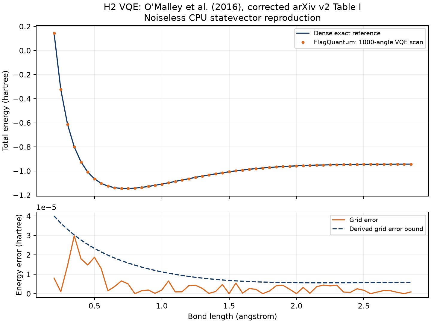
The figure is generated by this script, not copied from the paper. Reference CSV and recorded environment manifest are available for comparison. Small numerical differences across supported platforms are possible.

The largest scan error, about 2.98e-5 Eh, is below the paper's 1.6e-3 Eh chemical-accuracy scale relative to exact diagonalization of these rounded coefficients. This does not establish the hardware accuracy reported by the paper. The source's finer equilibrium R=0.72 angstrom is not a row of this 0.05-angstrom table; the best tabulated point is R=0.75. No interpolation or fitting is claimed here. Likewise, the endpoint at R=2.85 is a finite separation, not an independently established infinite-separation dissociation limit.

9. Additional Differentiable VQE Training

The original experiment scanned the parameter. This separate example demonstrates how the same paper model becomes a differentiable FlagQuantum training problem.

Mathematical operation	Code	Purpose
Initialize theta=0.2	torch.nn.Parameter(torch.tensor(0.2, dtype=REAL))	Start independently of the analytical minimizing angle.
$L(\theta)=E(\theta)$	loss = energy(theta, coefficients).mean()	A real scalar loss; there is no target-matching squared error.
$\nabla_\theta L$	loss.backward()	Differentiate the gate computation verified above.
Apply Adam	optimizer.step()	Tutorial optimizer; not a claim about the paper's experimental update rule.
Read the trained result	final = energy(theta, coefficients).squeeze(0)	Recompute after the last update, under no_grad.

Save as train_h2_vqe.py:

import torch
from h2_vqe_model import REAL, coefficients_at, energy, dense_hamiltonian

theta = torch.nn.Parameter(torch.tensor(0.2, dtype=REAL))
coefficients = coefficients_at(0.75)
optimizer = torch.optim.Adam([theta], lr=0.05)
initial = energy(theta, coefficients).item()
for _ in range(300):
    optimizer.zero_grad(set_to_none=True)
    loss = energy(theta, coefficients).mean()
    loss.backward()
    optimizer.step()

with torch.no_grad():
    final = energy(theta, coefficients).squeeze(0)
    exact = torch.linalg.eigvalsh(dense_hamiltonian(coefficients)).min()
    gap = (final - exact).item()
    assert -1e-10 <= gap < 1e-9
    print("Optimizer: Adam (tutorial extension; not the paper's 1000-angle scan)")
    print(f"Initial energy: {initial:.9f} Eh")
    print(f"Trained theta: {theta.item():.9f} rad")
    print(f"Post-update energy: {final.item():.9f} Eh")
    print(f"Exact reference: {exact.item():.9f} Eh")
    print("Energy gap below 1e-9 Eh:", abs(gap) < 1e-9)
    print("Differentiable VQE training checks passed.")

Run python train_h2_vqe.py. Output recorded in the verification environment:

Optimizer: Adam (tutorial extension; not the paper's 1000-angle scan)
Initial energy: -0.992295527 Eh
Trained theta: -0.114871869 rad
Post-update energy: -1.145599124 Eh
Exact reference: -1.145599124 Eh
Energy gap below 1e-9 Eh: True
Differentiable VQE training checks passed.

The assertion verifies the final energy against exact diagonalization with a 1e-9 Eh tolerance. The final angle's last digits can vary, and angles separated by pi give physically equivalent states. This successful bounded example is not a convergence guarantee for larger VQE problems.

10. Estimate Energy from Measurement Shots

The primary curve above uses exact expectations. To see how paper Eq. (4) becomes measured data, run a separate synthetic experiment at R=0.75 and the analytical minimizing angle. Three independent basis experiments suffice:

Basis / mathematical identity	Code before requesting samples	Terms recovered
Z basis	No additional gates	ZI, IZ, and ZZ from the same shots.
$H^\dagger ZH=X$	circuit.h(0).h(1)	XX from the product of two outcome signs.
$R_X(\pi/2)^\dagger ZR_X(\pi/2)=Y$	circuit.rx(0, math.pi/2).rx(1, math.pi/2)	YY from the product of two outcome signs.
$z_q=(-1)^{b_q}=1-2b_q$	signs = 1 - 2 * bits	Column 0 is logical q0; column 1 is q1.

The energy estimator is

$$\widehat E=c_I+\overline{V_Z}+\overline{V_X}+\overline{V_Y},\qquad V_Z=c_{ZI}z_0+c_{IZ}z_1+c_{ZZ}z_0z_1,\quad V_X=c_{XX}x_0x_1,\quad V_Y=c_{YY}y_0y_1.$$

Z terms share samples, so their covariance must be retained. Estimate each grouped per-shot energy first, then its variance. For independently seeded basis experiments with N shots each,

$$\widehat{\mathrm{SE}}(\widehat E)= \sqrt{\frac{s_Z^2+s_X^2+s_Y^2}{N}}.$$

Formula step	Code in sample_h2_energy.py
Compute a basis group's per-shot energy	per_shot = ... using the relevant coefficients and outcome signs.
Estimate variance of that group's mean	per_shot.var(unbiased=True) / shots
Add the constant and three group means	estimate = coefficients[0] + sum(means.values())
Combine independent group errors	standard_error = torch.sqrt(sum(variances.values()))

Save as sample_h2_energy.py:

import math
import torch
import flagquantum as fq
from h2_vqe_model import REAL, coefficients_at, ansatz, energy, analytic_minimum

coefficients = coefficients_at(0.75)
theta, _ = analytic_minimum(coefficients)
shots = 65536  # Per basis; three separately seeded basis experiments.
means, variances = {}, {}
for offset, basis in enumerate(("z", "x", "y")):
    circuit = ansatz(theta)
    if basis == "x":
        circuit.h(0).h(1)
    elif basis == "y":
        circuit.rx(0, math.pi/2).rx(1, math.pi/2)
    result = fq.run(circuit, outputs=fq.samples(name="bits"), shots=shots,
                    options=fq.ExecutionOptions(
                        mode="statevector", backend="pytorch", device="cpu",
                        precision="complex128", seed=2026+offset,
                        allow_backend_fallback=False, allow_approximate=False))
    bits = result.measurement("bits").value[0].to(REAL)
    assert bits.shape == (shots, 2)
    signs = 1 - 2 * bits
    if basis == "z":
        # ZI, IZ, and ZZ share shots: preserve their covariance.
        per_shot = (coefficients[1] * signs[:, 0]
                    + coefficients[2] * signs[:, 1]
                    + coefficients[3] * signs[:, 0] * signs[:, 1])
    else:
        coefficient = coefficients[4] if basis == "x" else coefficients[5]
        per_shot = coefficient * signs[:, 0] * signs[:, 1]
    means[basis] = per_shot.mean()
    variances[basis] = per_shot.var(unbiased=True) / shots
estimate = coefficients[0] + sum(means.values())
standard_error = torch.sqrt(sum(variances.values()))
exact = energy(theta, coefficients).squeeze(0)
error = (estimate - exact).abs()
assert error < 6 * standard_error + 1e-10
print("Synthetic simulator shots; no QPU or readout correction.")
print("Shots per basis / total:", shots, "/", 3 * shots)
print(f"Exact expectation: {exact.item():.9f} Eh")
print(f"Sampled estimate: {estimate.item():.9f} Eh")
print(f"Estimated standard error: {standard_error.item():.9f} Eh")
print("Absolute error below six estimated standard errors:", bool(error < 6 * standard_error))
print("Basis-rotation, shot-parity, and grouped-variance checks passed.")

Run python sample_h2_energy.py. Output observed with the recorded seeds/runtime:

Synthetic simulator shots; no QPU or readout correction.
Shots per basis / total: 65536 / 196608
Exact expectation: -1.145599124 Eh
Sampled estimate: -1.144471295 Eh
Estimated standard error: 0.000861071 Eh
Absolute error below six estimated standard errors: True
Basis-rotation, shot-parity, and grouped-variance checks passed.

Sampling outputs can differ across environments. The six-standard-error assertion is a broad statistical sanity check, not a guaranteed confidence interval or a chemical-accuracy guarantee. A finite-shot energy estimate may lie below the exact ground energy due to sampling fluctuation; the variational principle constrains the underlying expectation, not every noisy estimator. This experiment is separate from the exact 54-geometry scan and does not reproduce the paper's readout correction, gauge averaging, or device noise.

11. Verification Results and Reproduction Limits

Check actually executed	Result
Corrected Table I	54 rows, all six coefficients and geometry labels embedded; CSV hash verified.
Circuit translation at four angles	State matches both the analytical amplitudes and an independent matrix exponential, with rtol=atol=1e-10.
Five Pauli expectations and energy	Every term and the weighted scalar match the derivation and dense matrix reference.
Gradient	Autograd, closed-form, dense-exponential autograd, and explicit parameter shifts agree.
Full scan	All 54,000 energies match the derived energy surface; every grid minimum respects the variational and derived grid-error bounds.
Additional training	At R=0.75, 300 Adam updates reach the rounded-Hamiltonian ground energy within 1e-9 Eh.
Shot estimator	Z/X/Y basis rotations, outcome parity, grouped covariance handling, and the stated statistical check passed.

The numerical reference is the version-pinned, four-decimal Table I Hamiltonian. It is not an independent chemistry-integral calculation, an exact continuum molecular solution, or a replay of experimental photon/superconducting counts. Do not infer additional physical accuracy from printed nine-decimal simulation energies. Dense validation and the two-qubit ansatz are intentionally small; they establish no quantum advantage or large-system convergence claim.

A faithful hardware reproduction would additionally need the original native gates, calibration, readout corrections, gauge choices, statistical protocol, raw data, and optimizer/scan workflow. The paper's PEA/Trotterization experiment is outside this tutorial. For extending the workflow, use Noise and Open-System Simulation, Cloud and Quantum Hardware Execution, and Reproducibility and Benchmarks.

Sources and Citation

• O'Malley et al., Scalable Quantum Simulation of Molecular Energies, Physical Review X 6, 031007 (2016), DOI: 10.1103/PhysRevX.6.031007.
• Author-corrected arXiv v2 record, revised February 4, 2017; its revision note identifies the identity-coefficient correction. Version-pinned PDF: Eqs. (1)-(4), Fig. 1, Appendix A/B, and Table I on page 13 are the source of the model and transcription.
• Release circuit implementation, observables and requests, execution results.
• Documentation Guide: maintain formula/code pairings, independent checks, version labels, and actual browser verification.