Map products and field sampling
| Regional / SoilGrids workflow | Field-scale survey workflow |
|---|---|
 |
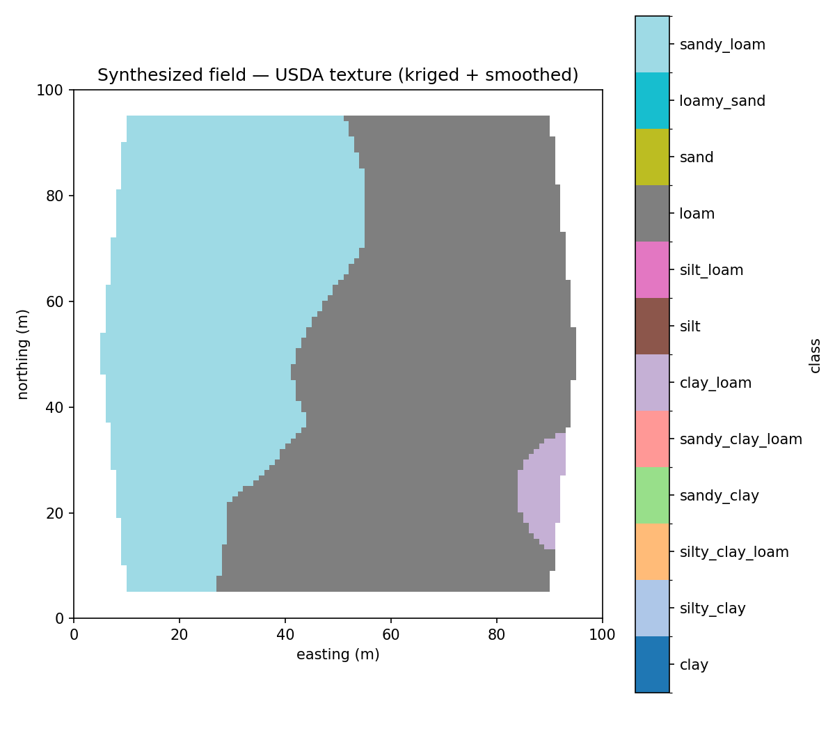 |
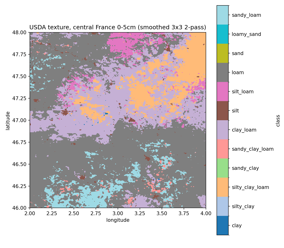
| 2°×2° SoilGrids tile, 740 745 pixels, USDA + 3×3 majority smoothing | 20 in-situ samples on a hexagonal field, kriged to a 1 m grid |
Two practical pipelines, both built on the same classify_array
core:
| Scenario | Input | Pipeline |
|---|---|---|
| Regional / world classification | Gridded sand/clay rasters (e.g. SoilGrids) |
classify_array → smooth_codes → write GeoTIFF + PNG + Shapefile |
| Field-scale survey | A handful of in-situ samples + a field boundary |
krige_sand_clay → classify_array → smoothing → same outputs |
This page walks both end-to-end and points out where each one benefits from the post-processing helpers added in pedotri 0.2.
Requires pedotri ≥ 0.2 (for
pedotri.rastermap-product helpers andpedotri.interpkriging). The interpolation path needs the[interp]extra; vector output needs[vector].
The input is two raster files (sand and clay) on the same grid. The output is a class-coded GeoTIFF, optionally smoothed, with vector and PNG companions for downstream use.
from pedotri.raster import classify_geotiff

codes, keys, profile = classify_geotiff(
    sand="sand_0-5cm_mean.tif",
    clay="clay_0-5cm_mean.tif",
    classification="USDA",
    units="g/kg",  # SoilGrids native units
)
codes is an int16 array (same shape as the input rasters) of
class indices into keys; -1 (pedotri.raster.NODATA_CODE) marks
invalid / masked pixels.
The raw classification can have salt-and-pepper artifacts at class boundaries — a single pixel of "sandy_loam" sitting inside a "loam" region usually reflects measurement noise rather than genuine spatial structure. The majority filter cleans these up:
from pedotri.raster import smooth_codes

smoothed = smooth_codes(codes, window=3, iterations=2)-
windowis the side length of the square neighbourhood (odd, ≥ 3). 3×3 is a conservative default; 5×5 absorbs slightly larger noise. -
iterationsre-applies the same filter; two passes converge for most natural raster noise patterns.
Nodata pixels are preserved (they neither vote nor get overwritten).
Implementation note: pedotri's smoother is the one-hot + box-filter
trick — for each class index, build a binary mask, run
scipy.ndimage.uniform_filter (C), then argmax across classes.
That's orders of magnitude faster than a Python-callback mode filter
on million-pixel rasters.
from pedotri.raster import (
    write_classified_geotiff,
    render_classified_png,
    classified_to_features,
    write_features_shapefile,
)

write_classified_geotiff("usda.tif", smoothed, profile=profile, keys=keys)
render_classified_png("usda.png", smoothed, keys=keys,
                      title="USDA — 0-5 cm", extent=(2, 4, 46, 48))
features = classified_to_features(smoothed, keys=keys,
                                   transform=profile["transform"],
                                   simplify_tolerance=0.005)
write_features_shapefile(features, "usda.shp", crs=str(profile["crs"]))
What you get:
-
usda.tif— paletteduint8GeoTIFF,nodata=255. QGIS picks up the color table automatically; class names are in band-1 GDAL tags asclass_0,class_1, … (see alsogdalinfooutput). -
usda.png— a categorical map with a side colorbar. Each class index gets a labeled tick. -
usda.shp— Shapefile with one (Multi)Polygon per contiguous class region; attributesclass_id(int) andclass_key(str). Pass.gpkg/.geojsonas the path suffix to get those formats instead (fiona auto-detects the driver).
The simplify_tolerance argument is in the CRS units of the raster
(degrees for WGS 84; metres for a projected CRS). For a SoilGrids
tile at 0.005° (~500 m at mid-latitudes) the polygons go from
hundreds of thousands of vertices to a few thousand without visible
loss of shape at viewing scale.
examples/soilgrids_france.py
runs the full pipeline against a 2°×2° SoilGrids tile of central
France. On a 2024 M-series Mac the classification takes ~0.12 s for
740 k pixels; smoothing adds ~0.3 s, polygonization adds ~0.3 s.
Now the input is a list of point samples (each with a measured sand %, silt %, clay %) and a polygon describing the field boundary. We want a continuous classified map of the field, even though we only sampled a handful of locations.
pedotri.interp.krige_sand_clay is the convenience wrapper:
from pedotri.interp import krige_sand_clay
from shapely.geometry import Polygon

samples = [
    {"x": 12.3, "y": 87.1, "sand": 42.0, "clay": 18.0},
    {"x": 25.0, "y": 35.0, "sand": 51.0, "clay": 22.0},
    # ... 20 in total
]
boundary = Polygon([(10, 5), (90, 5), (95, 50), (90, 95), (10, 95), (5, 50)])

sand_grid, clay_grid, profile = krige_sand_clay(
    samples,
    bbox=(0, 0, 100, 100),
    resolution=1.0,              # 1 m grid
    variogram="spherical",
    mask_polygon=boundary,
    crs="EPSG:32631",
)
Coordinate units (x, y, resolution) match the CRS — degrees
in lat/lon, metres in a projected CRS like UTM. The sample columns
are sand % and clay %; silt is implicit.
Pedotri uses ordinary kriging (via pykrige) for the
interpolation. The variogram is auto-fit from the samples; pick
"spherical" for typical soil texture, "linear" for tiny sample
sets, "gaussian" / "exponential" if you have a specific physical
reason. krige_samples (the lower-level function) also returns the
per-cell kriging variance — useful as a confidence map alongside
the prediction.
Cells outside mask_polygon come back as nan, and the downstream
classifier treats them as nodata.
The classification step from workflow A is unchanged — sand_grid
and clay_grid from kriging are just numpy arrays:
from pedotri.raster import classify_array, smooth_codes

codes, keys = classify_array(sand_grid, clay_grid, classification="USDA")
smoothed = smooth_codes(codes, window=3, iterations=2)
Then the same write_classified_geotiff / render_classified_png
/ write_features_shapefile triple as before.
krige_samples (the property-at-a-time helper used inside
krige_sand_clay) returns three things, not two:
from pedotri.interp import krige_samples

clay_grid, variance, profile = krige_samples(
    xs=[s["x"] for s in samples],
    ys=[s["y"] for s in samples],
    values=[s["clay"] for s in samples],
    bbox=(0, 0, 100, 100), resolution=1.0,
)
The variance grid is the kriging variance per cell: zero at sample
locations, larger away from them, very large outside the convex hull
of the samples. Treat it as your "this cell is mostly an
extrapolation" warning:
import numpy as np

confidence = 1.0 / (1.0 + variance)
codes = np.where(confidence > 0.5, codes, -1)  # mask low-confidence
For a serious field survey, report a bivariate confidence (combine the sand and clay variances) rather than the raw class map alone.
examples/field_kriging.py
synthesizes 20 samples on a hexagonal 100 m × 100 m field, krieges
sand and clay on a 1 m grid, masks to the boundary, classifies and
smooths under USDA, writes GeoTIFF + PNG + Shapefile.
-
No regression kriging. If you have a covariate (NDVI, DEM,
parent material map) and want to use it to improve the
interpolation, you need a different tool — pyKrige's
RegressionKriging, scikit-gstat, or a custom geostatistical pipeline. - No automatic variogram diagnostics. Pedotri uses pyKrige's auto-fit and doesn't second-guess it. For high-stakes work, inspect the empirical vs. fitted variogram in pyKrige before trusting the output map.
- No multi-band fusion. If you have sand, silt, clay all from a lab and want to honour the sum-to-100 constraint during interpolation, compositional kriging is the right answer; we krige sand and clay independently and accept the (small) inconsistency at the classification step.
-
No raster reprojection. All inputs to
classify_arrayandclassify_geotiffmust be on the same grid; reproject upstream withrasterio.warp/gdalwarp/rioxarray.reproject.
- GeoTIFF-and-SoilGrids — gridded-input flow with concrete SoilGrids URLs
- Classification-challenges — when you're choosing between systems or worried about cutoff drift
- API reference:
pedotri.raster,pedotri.interp(added in 0.2) - Examples:
examples/soilgrids_france.py,examples/field_kriging.py