Why multistart misses solutions

Why Multistart Misses Solutions

It seems logical that multistart is a good way to find alternative solutions to a large NLP: throw a hundred random starting points at the problem, collect the distinct minima, move on. The intuition is uncomfortable, though. A hundred points is a vanishing sample of a space with a thousand variables — so what exactly is multistart doing, and when does it stop working?

This page builds a problem where the answer is exact and checkable: a smooth NLP in n variables with exactly two minima, one a broad valley and one a narrow slot. Multistart finds the broad one and never the sharp one; deflation finds both in about five solves. Both facts are then explained quantitatively, including the conditions under which each conclusion would flip.

The short version:

Multistart's chance of finding a minimum is that minimum's basin measure under the sampler — nothing else. Dimension enters only through that measure. Deflation does not sample at all: it is a local continuation that escapes a known solution along the softest direction of its Hessian, and its cost is set by the landscape's geometry rather than by n.

---

A test problem with exactly two minima

The variables are the interior nodal values of a field u(x) on [0, 1] with u(0) = u(1) = 0, on n interior points with spacing h = 1/(n+1):

f(u) = ½ uᵀA u  +  W(u)

A = (1/h)·tridiag(-1, 2, -1) is the Dirichlet (smoothness) energy. Its eigenvectors are the sine modes φ_k = √2 sin(kπx) with S(φ_k) = k²π²/2. This is the broad valley: its minimum is u = 0, smooth deformations cost π² per unit amplitude, rough ones cost O(n²) more.

W digs one narrow, deep well at u* = a·φ₁:

W(u) = −D exp[ −(s−a)²/(2σ_s²) − ‖u − s·φ₁‖²/(2σ_r²) ],   s = ⟨u, φ₁⟩

with a = 0.5, D = 5, σ_s = 0.10, σ_r = 0.02, and box bounds u_i ∈ [−1, 1]. All norms are the L² (function-space) norm ⟨v,w⟩ = h Σ v_i w_i, so refining the grid is the same problem at higher resolution rather than a different problem.

σ_r ≪ σ_s makes the well a slot: to feel it at all, a point has to be a smooth field of very nearly the right shape.

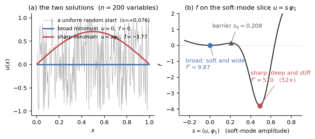
The two minima, at n = 200:

	broad	sharp
location	u = 0	u = 0.4903·φ₁
objective	0	−3.7903
curvature along φ₁ (L²)	π² = 9.87	π² + D/σ_s² = 510 — 52×
curvature along φ₂ (L²)	4π² = 39.5	4π² + D/σ_r² = 12 540 — 317×
Hessian eigenvalues (coefficient space)	0.049 … 804	2.54 … 866
width	none — an unbounded quadratic valley	σ_s = 0.10 along φ₁, σ_r = 0.02 in the other 199 directions
share of 5000 uniform starts	5000	0

The two are comparably stiff only in the roughest directions, where the Laplacian already dominates the well. In the smooth directions — the ones a solver actually travels along — the sharp minimum is one to two orders of magnitude tighter.

There are exactly two. Off the soft mode the quadratic dominates, and on the soft mode f(s) = π²s²/2 − D exp(−(s−a)²/2σ_s²) has exactly three stationary points — minimum, barrier, minimum — over any interval. Checked empirically as well: asking deflation, flooding and tunneling for six minima with a 60-solve budget, all three converge having found two, at every seed (verify.py). The barrier sits at s_b = 0.208, at height f = +0.143.

What actually happens

At n = 1000, with pounce driving the identical local solver in both cases:

method	solves	minima found	sharp found?	wall clock
multistart	200	1	✗	80.3 s
deflation	5	2	✓	3.0 s

Multistart is not merely slower — it does not find the second solution at all. Pushing the budget does not help: at n = 200, 5000 uniform starts return one minimum, 5000 times over.

The wall-clock column understates multistart's case, and it does not matter. Multistart is embarrassingly parallel, so those 80 s could be 1 s on 80 cores, while deflation is inherently serial — each solve starts from the previous minimum. The relevant number is not 200 solves but the number multistart would need, derived in why multistart fails: about 10²². No amount of parallelism reaches that.

Why multistart fails

The outcome of a solve is decided by one number

Project a starting point onto two coordinates: its amplitude in the soft mode, s = ⟨u₀, φ₁⟩, and its roughness, ρ = ‖u₀ − s·φ₁‖. Running a local solve from a grid of (s, ρ) and recording where it lands gives:

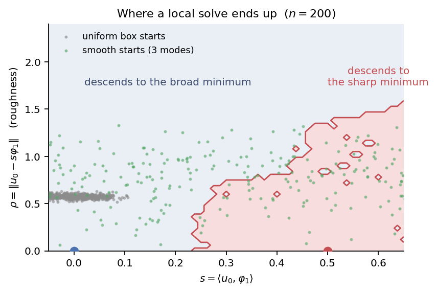
The boundary is steep. Roughness is largely forgiven — the solver contracts the stiff directions quickly — so the threshold drifts only from s ≈ 0.22 at ρ = 0 to s ≈ 0.5 at ρ = 1.5, and the basin closes off entirely only past ρ ≈ 2. A uniform random start has ρ = 0.574 ± 0.019, comfortably inside the tolerant range. Roughness is not what stops it. What decides the outcome is the soft-mode overlap s, and the sharp basin is essentially {s ≳ s_b}.

The grey cloud is 600 uniform starts. They form a tight band at s = −0.002 ± 0.041 — never within reach of the boundary, in any of 600 draws. The green cloud is the smooth sampler in multistart is not broken, at s = +0.05 ± 0.57, which straddles it.

(One caveat about this figure: it is a 2-D slice through a 200-D space, built along a single fixed rough direction. Other rough directions shift the boundary a little in both directions — which is exactly why the threshold is calibrated against measured hit counts below rather than read off this plot.)

Uniform sampling cannot produce that overlap

For u₀ uniform on [−1, 1]ⁿ,

s₀ = Σ_i h·φ₁(x_i)·u_i,     Var(s₀) = h²·Σφ₁² / 3 = h/3

because h Σ φ₁² = 1 by normalisation. So std(s₀) = √(h/3) → 0 as the grid is refined: a uniform random field is asymptotically orthogonal to any fixed smooth shape. (Measured: std(s₀) = 0.0403 at n = 200 against √(h/3) = 0.0407; over 20 000 draws the largest |s₀| was 0.156, never reaching s_b = 0.208.)

The hit probability is therefore

p(n) = P(s₀ > s_eff) ≈ Φ(−s_eff √(3(n+1)))

which decays exponentially in n — not because the box is large (nobody covers a box) but because the target's measure under the sampler collapses.

Calibrating the model

The geometric barrier s_b = 0.208 is a slight over-estimate of the effective threshold: a rough start is not confined to the soft-mode slice, and the extra directions give the solver room to round the barrier. Fitting s_eff by maximum likelihood to directly measured hit counts:

n	hits	starts	measured rate	s_eff implied by this n alone
20	72	2 000	3.6e-02	0.227
35	61	3 000	2.0e-02	0.197
60	23	3 000	7.7e-03	0.179
100	5	5 000	1.0e-03	0.178
150	1	6 000	1.7e-04	0.169
200	0	5 000	0	—

The implied threshold settles by n ≈ 60. The pooled maximum-likelihood fit over n ≥ 60 gives s_eff = 0.178, against the geometric barrier s_b = 0.208. The model therefore has exactly one fitted number, and all of the n-dependence comes from std(s₀) = √(h/3). That s_eff < s_b says the effective basin is slightly larger than the soft-mode slice suggests: averaged over rough directions, a few of them help the solver round the barrier more than the rest hinder it.

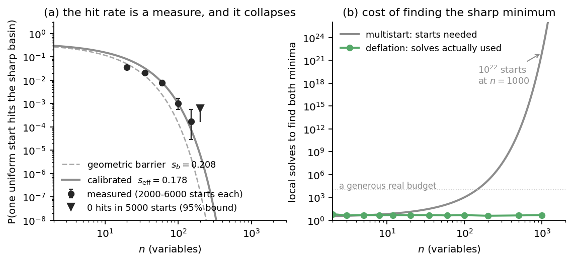
Extrapolating the calibrated model — and, for comparison, the uncalibrated geometric one:

n	P(hit) calibrated	starts needed	P(hit) geometric
100	9.9e-04	1.0e+03	1.5e-04
200	6.3e-06	1.6e+05	1.6e-07
500	2.7e-12	3.7e+11	3.7e-16
1 000	9.9e-23	1.0e+22	2.1e-30
2 000	1.8e-43	5.5e+42	9.9e-59
10 000	1.5e-208	6.6e+207	1.5e-284

At n = 1000 — the headline problem — uniform multistart needs of order 10²² starts. Deflation needs 5. The gap is not a constant factor that parallelism or a faster local solver can close.

The transition, measured

Sweeping n with 200 starts per seed, 5 seeds — and deflation on the same problems:

n	multistart: seeds finding sharp	mean solves	deflation: seeds finding sharp	mean solves
2	5/5	12.0	5/5	6.2
5	5/5	43.2	5/5	4.6
12	5/5	14.0	5/5	4.6
20	5/5	46.6	5/5	4.6
35	5/5	69.4	5/5	4.6
60	5/5	80.4	5/5	4.2
100	1/5	179.0	5/5	4.6
200	0/5	200 (budget)	5/5	3.8
500	0/5	200 (budget)	5/5	4.2
1 000	0/5	200 (budget)	5/5	4.6

Deflation's solve count is flat in n — 4.6 solves at n = 1000, the same as at n = 5. Multistart's climbs until it hits the budget and then simply stops finding anything.

Multistart is not broken at n = 20; it is fine there, and it degrades smoothly. This is why low-dimensional pictures mislead: the same landscape, drawn in 2-D, would make multistart look perfectly adequate.

Why deflation succeeds

Pounce's deflation restarts each solve from the last minimum found, not from a random point. It is a local continuation, and that is the whole difference. Adding the pole at the known minimum u = 0,

F(u) = f(u) + η / (‖u‖/ℓ)²

the cheapest way out is the direction of least curvature. Restricted to the soft mode with stiffness λ = π², minimising ½λs² + ηℓ²/s² gives an escape radius

s* = (2ηℓ²/λ)^(1/4)

With η = 1, ℓ = 0.2: s* = 0.3001. Solving the deflated problem directly and decomposing the result in the mode basis:

escaped to s = ±0.3000,  mode content |c_k| = [0.3000, 0, 0, 0, 0, 0, 0, 0]

The escape is pure mode 1 — every other coefficient is zero to machine precision — at the predicted radius to four digits. Since s* = 0.300 clears the barrier s_b = 0.208, the polish step on the clean objective falls into the sharp well.

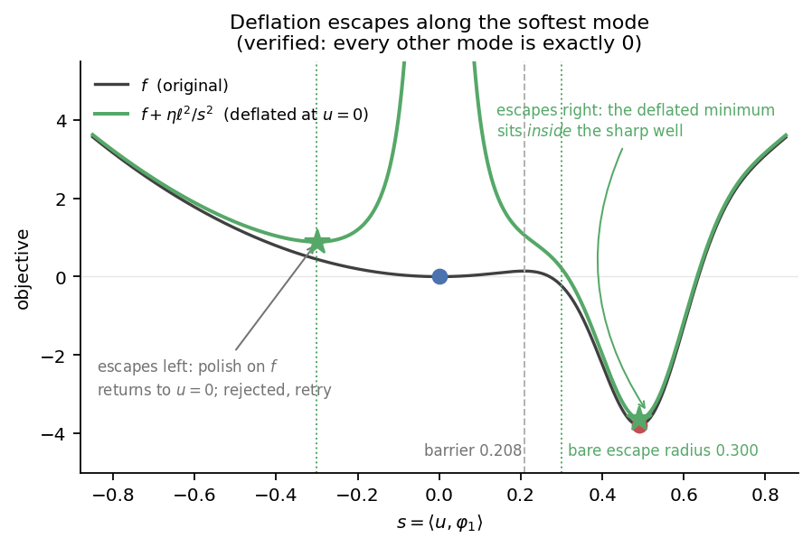
That also explains why deflation takes ~4 solves rather than 2: the escape sign is a coin flip. Escaping to s = −0.300 lands nowhere — the polish returns to u = 0, the candidate is rejected as already known, and the search retries. Each retry is another ~50 % chance.

The success condition, stated correctly

It is tempting to say deflation works when the escape radius clears the barrier, s* > s_b. That is sufficient but not necessary, and the truth is more forgiving. What matters is whether the deflated objective F has a spurious local minimum on the escape ray, short of the target:

pole radius ℓ (L²)	bare escape s*	spurious minimum of F at	outcome
0.005	0.047	0.048	trapped
0.0141 — pounce's default at n=200	0.080	0.081	trapped
0.030	0.116	0.120	trapped
0.045	0.142	0.155	trapped
0.050	0.150	none	slides into the well
0.200	0.300	none	slides into the well

Below ℓ ≈ 0.05 the pole leaves a stationary point of F at the escape radius; the solver converges there (|∇F| ~ 10⁻⁸ — this is a real minimum, not a premature stop), the polish on f returns to u = 0, and the candidate is rejected as already known. Above it, the well's attraction already exceeds the quadratic's restoring force at the escape radius, no stationary point survives in between, and the deflated solve runs straight into the sharp minimum.

Note the threshold sits at s* ≈ 0.15, inside the barrier at s_b = 0.208: the deflated problem is easier to escape than the original one, because the pole tilts the barrier away. Measured over 5 seeds with a 40-solve budget, deflation finds the sharp minimum for every ℓ from 0.05 to 0.8 (~4 solves) and fails for every ℓ ≤ 0.014.

This is a statement about geometry, not about dimension — which is why the solve count in the sweep above is flat in n.

Deflation is not magic: the pole must be sized in the right metric

Pounce sizes repulsion widths as a fraction of each variable's bounds range, in the Euclidean norm of the coefficient vector. On a grid problem that is the wrong norm: ‖u‖_euclid = ‖u‖_L2 / √h, so a pole of fixed coefficient-space radius shrinks like √h in function space. Refine the grid and the pole quietly becomes too weak to escape anything.

n	default pole radius (in L²)	escape s*	minima found	solves	L² pole radius	escape s*	minima found	solves
100	0.0199	0.095	1	20	0.20	0.300	2	3
200	0.0141	0.080	1	20	0.20	0.300	2	3
500	0.0089	0.063	1	20	0.20	0.300	2	5
1 000	0.0063	0.053	1	20	0.20	0.300	2	5

With the default scaling the escape radius never reaches the barrier s_b = 0.208, at any n, and it gets worse with refinement — deflation returns one minimum and burns its whole budget. In the L² metric the escape radius is grid-independent and clears the barrier every time.

The fix is two arguments — measure distances and size the pole in the problem's own norm:

result = pounce.find_minima(
    f, u0, method="deflation", jac=jac, hess=hess, bounds=bounds,
    n_minima=2,
    distance=lambda a, b: l2(a, b),          # L2, not coefficient Euclidean
    strategy_kw={"length": 0.2 / np.sqrt(h)},   # pole radius 0.2 in L2
)

This is the single most important practical detail on this page. Every "deflation didn't work" result here came from leaving it out.

Sharpness is the knob

Sharpness does not enter the hit probability directly — it enters through the barrier. A wide well reaches back toward the incumbent solution and puts its barrier close to the origin, so a start needs only a small soft-mode overlap. A narrow well pushes the barrier out. Sweeping the well width σ_s at fixed depth and position:

σ_s (well width)	curvature at the sharp minimum	barrier s_b	P(hit), n=200	P(hit), n=1000	two minima?
0.04	15.6	0.378	7.6e-21	8.4e-96	yes
0.06	6.96	0.323	1.1e-15	1.9e-70	yes
0.08	3.94	0.267	2.6e-11	7.2e-49	yes
0.10	2.54	0.208	1.6e-07	2.1e-30	yes
0.12	1.78	0.140	3.0e-04	9.9e-15	yes
0.13	1.52	0.095	9.7e-03	9.0e-08	yes
0.14	1.41	—	0.5	0.5	no — one minimum
0.25	0.45	—	0.5	0.5	no — one minimum

(Probabilities here use the geometric barrier, so they are the conservative column; the calibrated numbers are ~30× larger and change nothing.)

Two things worth reading off this table. First, the chain is monotone: sharper well → barrier further out → hit rate collapses. Second, σ_s = 0.10 is close to the most findable configuration that still has two minima — past σ_s ≈ 0.135 the well's tail swallows the broad minimum and only one remains. The problem above is therefore about as favourable to multistart as a genuine two-minimum instance of this family can be.

Multistart is not broken, uninformed sampling is

The failure is a property of the sampler, not of the restart strategy. Draw starts from the K softest modes instead,

u₀ = Σ_{j≤K} c_j φ_j,   c_j ~ U(−1, 1)

and ⟨u₀, φ₁⟩ = c₁ has spread 1/√3 for every n. The hit rate then stops depending on n at all:

Hit rate vs. how many modes you sample (n = 200, 300 starts each):

K	hits	rate
1	108/300	0.360
2	47/300	0.157
3	35/300	0.117
5	20/300	0.067
10	13/300	0.043
25	0/300	0.000

K = 1 sits just under its ceiling P(c₁ > s_b) = 0.396. Adding modes adds roughness, which erodes the rate slowly — and kills it at K = 25, where ρ ≈ √(24/3) = 2.8 finally exceeds the roughness tolerance the basin map showed at ρ ≈ 2.

Hit rate vs. n, at a fixed K = 3, next to uniform sampling on the same problems with the same solver:

n	smooth (K=3)	uniform	uniform, predicted
20	43/200 = 0.215	5/200	5.0e-02
60	36/200 = 0.180	1/200	2.5e-03
200	28/200 = 0.140	0/200	1.6e-07
500	7/60 = 0.117	0/60	3.7e-16
1 000	5/60 = 0.083	0/60	2.1e-30

At n = 1000: 8 % per start from three smooth modes, versus one chance in 10²² from uniform noise. Identical problem, identical local solver, identical restart strategy — only the sampling basis differs. In the (s, ρ) plane the reason is immediate: uniform starts land in a tight blob at s = −0.002 ± 0.041, while the smooth sampler spreads over s = +0.05 ± 0.57, straddling the barrier.

This is the constructive reading of the whole page. Multistart's cost is set by the measure of the target basin under your sampler; you can fix it by changing the sampler, if you know enough about the problem to align it with the directions that decide the outcome. Deflation's appeal is that it gets that alignment for free — the Hessian at the incumbent solution already knows which directions are soft.

Which of the six strategies is best?

The first cut is by family and it is absolute: the three repulsion methods find the sharp minimum, the two restart methods and basinhopping never do. But that is only a fair comparison if each method's scale knob is tuned, so every method was swept over a wide range at n = 200 (5 seeds, 40-solve budget) and scored on its best setting.

The three that work

method	knob	working range (L²)	hits	solves	wall clock n=200	wall clock n=1000
deflation	length	0.05 – 0.8	5/5	3.8	0.07 s	3.1 s (5.7 solves)
flooding	sigma	0.05 – 0.8	5/5	7.0	0.12 s	5.6 s (7.7 solves)
tunneling	length	0.1 – 0.5	5/5	5.0	18 s	did not finish in 15 min

Deflation wins on cost — about half the solves of flooding, and ~2× less wall clock at n = 1000. Their robustness is nearly identical. Swept down to a width of 0.005, both fail below 0.02 and both are reliable from 0.05 up:

width (L²)	0.005	0.01	0.02	0.03	0.04	0.05	0.07
deflation hits	0/5	0/5	2/5	2/5	4/5	5/5	5/5
deflation solves	40	40	34.0	27.2	20.8	4.2	4.2
flooding hits	0/5	0/5	1/5	4/5	4/5	5/5	5/5
flooding solves	40	40	33.8	22.0	23.6	12.2	8.6

Flooding is slightly better in the marginal band (4/5 vs 2/5 at width 0.03), because it raises its bump adaptively when a solve falls back into a flooded basin, whereas deflation's pole is static. Above the threshold deflation is markedly cheaper. There is no width at which flooding finds it and deflation cannot.

Tunneling works but is ~250× slower per solve. It minimises a merit function that pounce differentiates by finite differences — O(n) extra evaluations per iteration, with no way to supply an analytic gradient. Each evaluation is itself O(n²) on this problem, so a run scales as O(n³): going from n = 200 to n = 1000 predicts 125×, i.e. 18 s becoming ~37 min. A single n = 1000 run was abandoned after 30 minutes without finishing, which is consistent. It is the wrong tool for a large problem unless you specifically want its monotonically descending trail of minima.

The three that don't — and each fails for a different reason

multistart — the measure argument in why multistart fails.

basinhopping — fails at every step size tested, 0.1 through 5.0, 0/5 each. Its proposal is x + step·N(0, I), isotropic in coefficient space, so a step's soft-mode overlap has std = step·√h — the same √h collapse that kills uniform sampling. Worse, the box clip saturates it: past step ≈ 1 every coordinate pins to ±1, a box corner, whose overlap std is exactly √h no matter how much larger step gets. There is no setting that works. A proposal that could work would have to be anisotropic, biased toward the soft modes — which means already knowing the answer.

mlsl — fails twice over.

1. Its sampler is multistart's. MLSL draws uniformly from the box and then decides whether to start a solve from each sample. The filter can only remove solves, never reach new points, so its discovery can never exceed multistart's. Its ordering heuristic — solve from the lowest-f samples first — carries no signal here either: for a random start f is dominated by roughness (13 414 ± 1297) while the soft mode contributes 0.008 of it, giving corr(f(u₀), s₀) = −0.004. Among the 400 lowest-f of 4000 starts the largest |s₀| was 0.132, still short of the 0.208 barrier.
2. Its clustering radius degenerates in high dimension. The reduced distance is γ·√n·(log N / N)^(1/n), and (log N/N)^(1/n) → 1 as n grows, so the radius saturates at γ·√n while the typical distance between two scaled samples is √(n/6):

n	(log N/N)^(1/n)	radius	typical pair distance	ratio
2	0.215	0.61	0.58	1.05
20	0.857	7.67	1.83	4.20
200	0.985	27.9	5.77	4.82
1 000	0.997	63.1	12.9	4.88

The ratio saturates near 4.9 for every n ≥ 20, so every fresh sample is "near" the one known minimum, is filtered, and no local solve ever fires. With the default γ = 2, MLSL does exactly 1 solve and stops. Turning γ down to 0.02 restores the solves and it becomes multistart again (0/5). This looks like a genuine defect of the reduced-distance rule at large n rather than a tuning problem: the shrink factor that is supposed to tighten the radius as the pool grows has essentially no effect once n is large.

Summary

Use deflation, with the L² scaling from sizing the pole. flooding is a near-equal alternative and marginally more forgiving of a too-narrow width. tunneling only if you want its descending trail and can afford finite-difference gradients. The restart and hopping methods are not merely worse tuned here — they are structurally unable to find this solution, because all three propose points isotropically in a space whose one relevant direction occupies a vanishing fraction of it.

What to take away

1. The right mental model is measure, not coverage. With N uniform starts, P(find) ≈ N·p, where p is the basin's share of the sampler. You need N ~ 1/p. Nobody ever covers a high-dimensional box, and that was never the mechanism.
2. Dimension only matters through p. Multistart is fine in 1000 variables when every basin is fat in every direction, and hopeless in 60 when one is not. Count the directions in which the basin is thin, not the variables.
3. The classical guarantees are asymptotic, and asymptotics are not a budget. Multistart and MLSL are correct in the limit: sample forever and you find every minimum with probability 1 (Rinnooy Kan & Timmer, 1987). What that says nothing about is how many samples, and the answer is 1/p. Here 1/p = 10²². The theorem is true and useless, and nothing in the method's output warns you which regime you are in.
4. Deflation trades a measure problem for a geometry problem. It always escapes along the softest Hessian direction at the incumbent, and finds whatever lies there. That is dimension-independent, and it is also a real limitation: put the second minimum somewhere that is not reachable along a low-curvature escape, and deflation will miss it too. It is not a global search.
5. The failure is shared by every method that proposes points isotropically. multistart, mlsl and basinhopping all fail here, at every setting of every knob, for the same underlying reason — not because they are badly tuned. Any method whose proposal is isotropic in coefficient space inherits the √h collapse. What distinguishes the repulsion methods is not that they sample better; it is that they do not sample at all.
6. Scale the pole in the problem's metric. On discretised problems the default coefficient-space scaling silently weakens with refinement.
7. Absence of evidence is weak evidence here. "I ran 100 multistarts and found one solution" is compatible with there being exactly one solution, and equally compatible with there being a second one you would need 10²² starts to see. Multistart cannot distinguish those two cases, and it does not tell you which one you are in.