Cape Fox Simulator
Cape Fox is a simulator build as an extension to TinyOS's TOSSIM simulator.
Besides TOSSIM functionality, Cape Fox also provides:
- support for simulation of the MAC protocol source code implementation
- integration with TOSSIM Live extension
- interface for inserting real-time sensor data or sensor data traces
- interface for reading actuation signals
- support for execution of the Fennec Fox protocol stack
The Cape Fox source code comes with Fennec Fox. It is located in src/support/cape. Examples of the simulator control scripts can be found in sim directory.
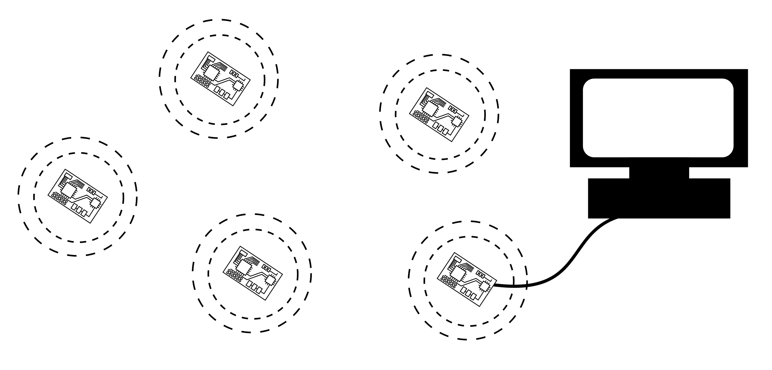
Testing and debugging embedded firmware running on a network of motes can be time consuming. Many software design decisions and implementation issues can be evaluated and corrected while running the code in a simulator. The following steps show how to test a Swift Fox program collecting sensor measurements over a multihop mesh network at a single mote (called sink) that forwards all the sensor measurements to a PC. The figure below shows a sketch of the target system that we want to implement.
The system presented on the figure above can be programmed in Swift Fox with the following code:
configuration sense { telosSens(5, 1024)
                        ctp(5)
                        csmaca(5, 0, 10, 10, 1, 1, 1)
                        # always ON, delay_after_receive, backoff, min_backoff
                        # ack, cca, crc
                        cc2420(26, 31, 1, 1)
                        # channel, power, ack, crc
                        }

state test { sense }

start test
In this program we assume that the Fennec Fox application module collects measurements from the sensors that are on the TelosB motes. At the picture above, the sink mote is the mote attached through the serial cable to a PC, and it has address ID 5. Sensors' measurements are collected every 1024ms, and they are forwarded to the sink mote (ID 5) over the CTP data collection network protocol. Because TelosB motes use CC2420 radio chip for the wireless communication, the Swift Fox sense network process uses the cc2420 radio driver, sending packets on the channel 26, with the maximum (31) signal strength (0dBm).
Before we program and test the code that is running on the motes, we may want to test it in a simulator. In Cape Fox simulator we will be able to test the top three layers of the stack, i.e. the application, network and MAC layers. This means that the same code that will run on these layers in the final hardware implementation is the same code that we can test in the simulator. In the sensor measurements collection application there are two differences between the actual hardware code implementation and the code that we can test in the simulator:
- we simulate the wireless radio communication
- we simulate sensor measurements
That is, every part of the Wireless Sensor Network or a Cyber-Physical System that is interacting with the surrounding environment must be simulated. Thus, we simulated wireless communication and simulate sensor measurements.
First, let's look at the example of the Swift Fox code above and its modification to enable Cape Fox simulation:
configuration sense { telosSens(5, 1024)
                        ctp(5)
                        csmaca(5, 0, 10, 10, 1, 1, 1)
                        # always ON, delay_after_receive, backoff, min_backoff
                        # ack, cca, crc
                        cape()
                        }

state test { sense }

start test
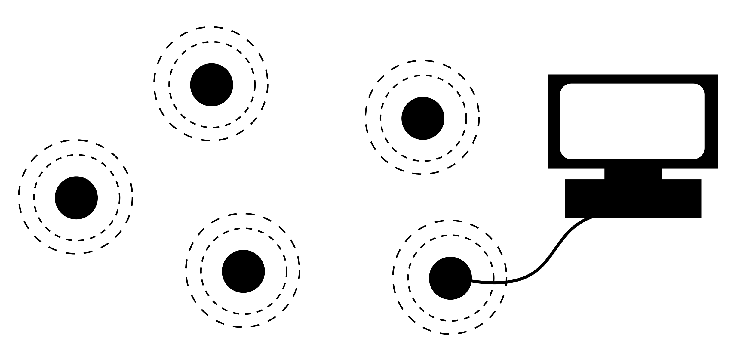
Noticed the difference on the radio layer of the sense network process: instead of using the cc2420() radio driver, the process runs on the cape() radio driver, a code that links to the simulator's model of wireless communication. Switching the radio driver from the one specific to the target platform architecture into the cape() is everything that is needed to let the Swift Fox program to be successfully tested in the Cape Fox simulator. Thus, now we can imagine that instead of running actual wireless network, we simulate a network as the one shown on the figure below.
Another difference between the actual system deployment and the simulated network scenario is the sensor data generation. In the real deployment, the embedded firmware accesses the hardware sensors to get the measurements, while in the simulated system, the sensor measurements are fed into the simulator.
First, let's look into the implementation of the telosSens application. The source code of this application is stored in src/Application/tests/TelosbSensors. The top configuration file of this application is TelosbSensorsC.nc. Looking into this file we see the following lines of code:
#ifndef TOSSIM

components new SensirionSht11C();
TelosbSensorsP.ReadHumidity -> SensirionSht11C.Humidity;
TelosbSensorsP.ReadTemperature -> SensirionSht11C.Temperature;

components new HamamatsuS10871TsrC();
TelosbSensorsP.ReadLight -> HamamatsuS10871TsrC;

#else

components new CapeInputC() as CapeHumidityC;
TelosbSensorsP.ReadHumidity -> CapeHumidityC.Read16;

components new CapeInputC() as CapeTemperatureC;
TelosbSensorsP.ReadTemperature -> CapeTemperatureC.Read16;

components new CapeInputC() as CapeLightC;
TelosbSensorsP.ReadLight -> CapeLightC.Read16;

#endif
From this code we learn the following. First, the application's implementation module TelosbSensorsP.nc is using ReadHumidity, ReadTemperature, and ReadLight interfaces to connect to the sensors. Each of those interfaces is of type Read< uint16_t >. The #ifndef TOSSIM and #else ... #endif are include guards that specify when the application module should wire to the actual sensors' drivers and when it should wire into the simulated sensor drivers. When the code is not compiled into TOSSIM simulator, the module wires to SensirionSht11C and HamamatsuS10871TsrC sensors' drivers. When the code is compiled for simulation, the TelosbSensorsP.nc wires into generic simulated Cape Fox data input streams CapeInputC. Then, during the simulation, the CapeInputC retrieves simulated measurements from the Cape Fox simulator.
Next we look into the steps necessary to compile and run an instance of Cape Fox simulation. Let's say that the above Swift Fox program (the one with cape() as the radio driver) is saved in a file called telosB_cape.sfp. Then, we can compile this program as follows:
user@linux $ sfc telosB_cape.sfp
user@linux $ fennec micaz cape
The second line follows the TOSSIM compilation procedure, which targets micaz architecture.
Once the program is compiled we can run the simulation. In the src/support/cape/sim directory there is a set of Python script examples that can run a simulation. These Python scripts follow the TOSSIM simulation model, i.e. the scripts use the same mechanisms to: generate the simulated network topology, create wireless communication noise traces, and inspect each simulated mote status.
When entering the src/support/cape/sim directory for the first time, run make to create various network topologies and noise traces:
user@linux $ pwd
.../src/support/cape/sim
user@linux $ make
One can create its own simulated network topologies by following TOSSIM tutorial and using the tools to build network topologies for TOSSIM.
First we look how to run a fast Cape Fox simulation. In the first example, we use the following Swift Fox program:
uint16_t dest_node = 2
uint16_t src_node = 0xFFFF

configuration count {
                        counter(10, 1024, src_node, dest_node)
                        ctp(dest_node)
                        csmaca(dest_node, 0, 10, 10, 1, 1, 1)
                        # always ON, delay_after_receive, backoff, min_backoff
                        # ack, cca, crc
                        cape()
}

state simple_sim { count }

start simple_sim
This code is a modified version of the code example presented above, with the telosSens application substituted with counter Fennec Fox application module. This application instead of sending sensor measurements to the destination node, it sends a message with a counter that is increased by 1 after each transmission. If we save this program in counter_cape.sfp file, then we can compile it as follows:
user@linux $ sfc counter_cape.sfp
user@linux $ fennec micaz cape
Next, we go to the src/support/cape/sim directory and run
user@linux $ ./fastSim.py
Which will run the Cape Fox simulator, following the fastSim.py script. In this script we see that the simulation is set with the following parameters:
		self.dbg_channels = ["Application", "Network"]
		self.cape.setTopologyFile("topos/4/linkgain.out")
		self.cape.setNoiseFile("noise/casino.txt")
		self.cape.setSimulationTime(200)
These parameters say that the simulator should record all dbg() statements from the tested embedded firmware that are send to Application and Network debugging channels. For example, in src/Application/tests/Counter/CounterP.nc we see the following lines of code:
	dbg("Application", "Counter SplitControl.start()");

	dbg("Application", "Counter starting delay: %d", send_delay);
	dbg("Application", "Counter starting src: %d  dest: %d",
		call CounterParams.get_src(), call CounterParams.get_dest());
The fastSim.py also sets the network topology to a 2-by-2 grid, with total of 4 motes. The radio noise simulation follows the model from the casino.txt file, and the simulation runs for 200 seconds.
After running the simulation:
user@linux $ ./fastSim.py
we will find dbg statements in src/support/cape/sim/results folder. A sample set of dbg logs may look like this:
         0 000 000 NODE (0000): ctpP SplitControl.start()
         0 000 000 NODE (0000): CtpRoutingEngineP StdControl.start()
         0 000 000 NODE (0000): ctpP SplitControl.start() - root: 2
         0 000 000 NODE (0000): Counter SplitControl.start()
         0 000 000 NODE (0000): Counter starting delay: 10240
         0 000 000 NODE (0000): Counter starting src: 65535  dest: 2
         0 020 000 NODE (0001): ctpP SplitControl.start()
         0 020 000 NODE (0001): CtpRoutingEngineP StdControl.start()
         0 020 000 NODE (0001): ctpP SplitControl.start() - root: 2
         0 020 000 NODE (0001): Counter SplitControl.start()
         0 020 000 NODE (0001): Counter starting delay: 10240
         0 020 000 NODE (0001): Counter starting src: 65535  dest: 2
         0 040 000 NODE (0002): ctpP SplitControl.start()
         0 040 000 NODE (0002): CtpRoutingEngineP StdControl.start()
         0 040 000 NODE (0002): ctpP SplitControl.start() - root: 2
         0 040 000 NODE (0002): Counter SplitControl.start()
         0 040 000 NODE (0002): Counter starting delay: 10240
         0 040 000 NODE (0002): Counter starting src: 65535  dest: 2
         0 060 000 NODE (0003): ctpP SplitControl.start()
         0 060 000 NODE (0003): CtpRoutingEngineP StdControl.start()
         0 060 000 NODE (0003): ctpP SplitControl.start() - root: 2
         0 060 000 NODE (0003): Counter SplitControl.start()
         0 060 000 NODE (0003): Counter starting delay: 10240
         0 060 000 NODE (0003): Counter starting src: 65535  dest: 2
         0 110 351 NODE (0000): Network CTP send beacon message
where the first column is the simulated time (< minutes > < seconds > < milliseconds >), followed by the mote address and followed by the dbg statement.
In this example we will run a real-time simulation. First, we will simulate a network with motes collecting sensor measurements in a real-time, and with the sink node sending the sensors' reports to serial interface also in the real-time. Then, we will enhance this example with a simulation that remotely feeds sensor measurements into the simulator running in real-time.
Real-Time simulations are particularly important in developing and testing Cyber-Physical Systems. For example, we might want to build a Cyber-Physical System as the shows on the figure below:
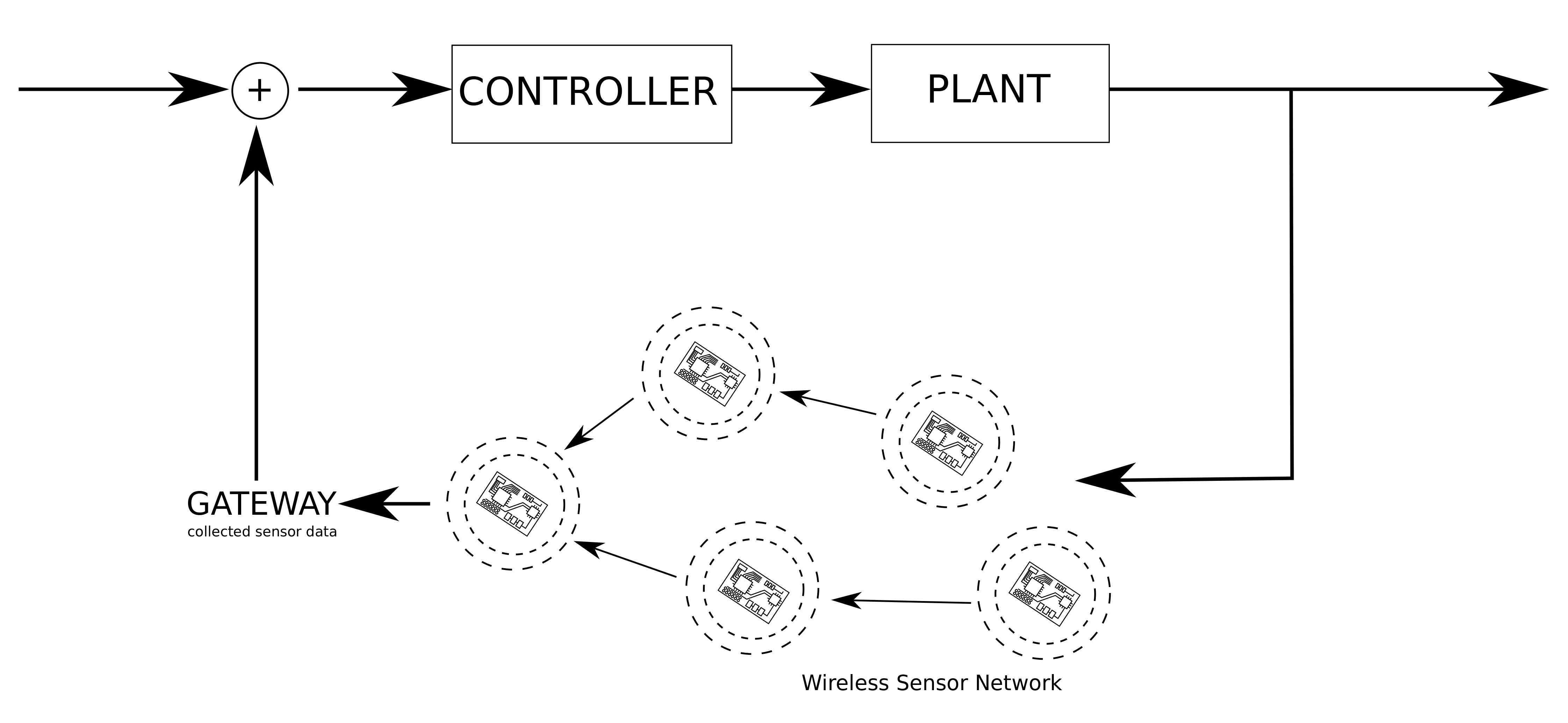
In the figure above, we show a control system, with a controller actuating on a plant. The controller makes its decisions based on the sensors' measurements that are collected by a Wireless Sensor Network.
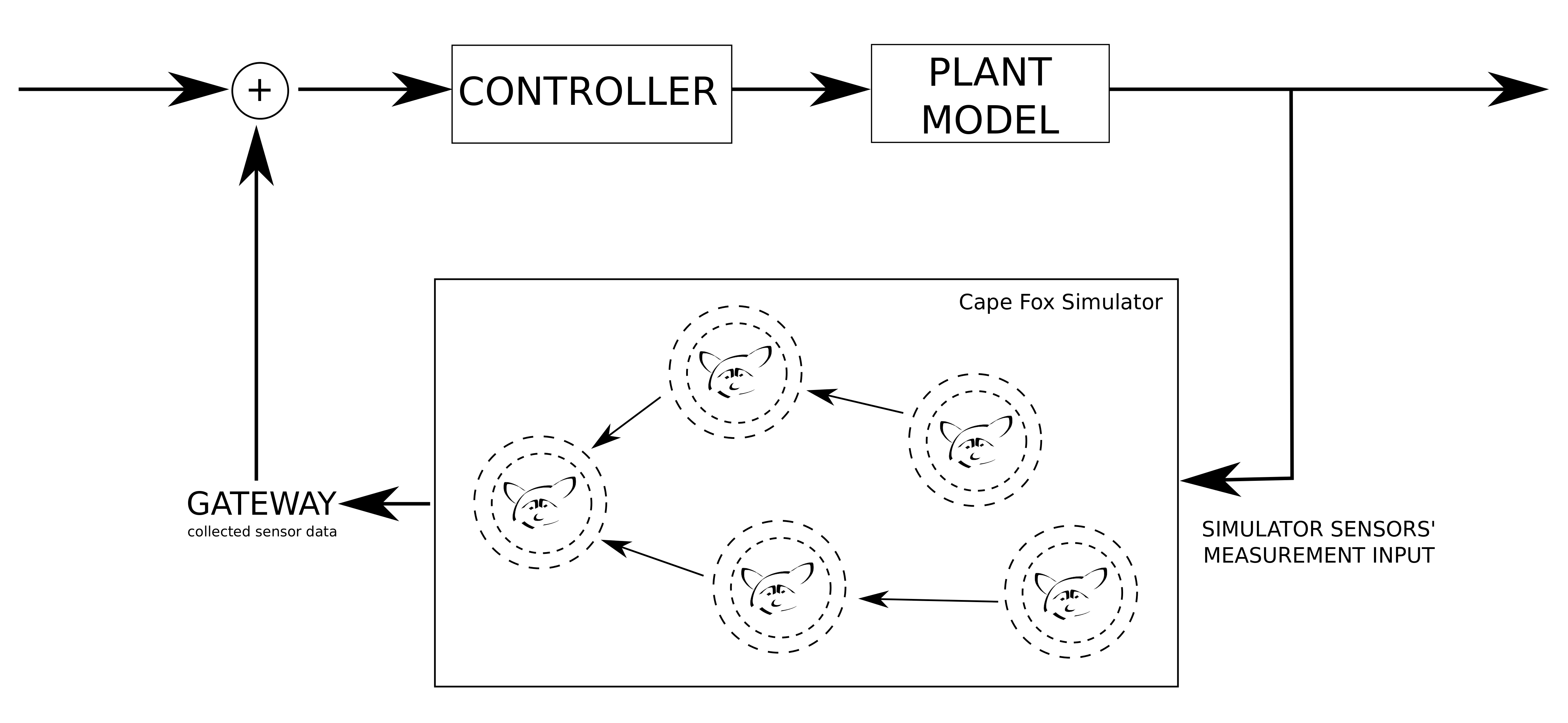
Before we deploy a Cyber-Physical System, we might want to test the implementation of the Wireless Sensor Network together with the implementation of a controller actuating on a model of a plant. During the system simulation the model of the plan generates sensors measurements that are fed into the Cape Fox simulator, as shown on the figure below.
In the following example, we look how to simulate a Cyber-Physical System, where Wireless Sensor Network collects measurements from the sensors located on the TelosB motes. We can reuse the previous Swift Fox code that collects sensors' measurements from TelosB motes. This program looks as follows:
configuration sense { telosSens(1, 1024)
                        ctp(1)
                        csmaca(1, 0, 10, 10, 1, 1, 1)
                        # always ON, delay_after_receive, backoff, min_backoff
                        # ack, cca, crc
                        cape()
                        }

state test { sense }

start test
After compiling this code, we can run a real-time simulation using the realTimeSim.py Python script.
In one window shell, we run the script as follows:
user@linux $ ./realTimeSim.py
This will run the simulation, with the simulate time advancing according to the real clock of the computer that runs the simulation. During the execution, all dbg channels that are enabled will be generating log statements in the results directory.
Because telosSens application sends messages over the serial connection, we can see those messages by running another Python script that connects to the TinyOS serial forwarder set up by the Cape Fox simulator. In the second window shell, we run UARTGatewayTelosb.py Python script that follows TinyOS's API of connecting to Serial Forwarder:
user@linux $ ./UARTGatewayTelosb.py
This will connect to the network port at the computer that runs the simulation. On this connection, the script will receive serial messages and parse them according to the message structure definition specified in the TelosbSensors.h TelosbSensors application. The following are examples of the output printed by the UARTGatewayTelosb.py script:
1393206961.47 1 0 0 0 0
Message <TelosbMsg>
  [seq=0x0]
  [src=0x2]
  [hum=0x0]
  [temp=0x0]
  [light=0x0]

1393206962.17 2 0 0 0 0
Message <TelosbMsg>
  [seq=0x0]
  [src=0x3]
  [hum=0x0]
  [temp=0x0]
  [light=0x0]
In this simulation, at run-time Cape Fox generated a set of sensors' measurements. The sensors' measurements are computed by the simulatedData function, implemented as follows:
uint32_t simulateData(uint16_t node_id, uint8_t io_id, long long int time_val) {
	return (io_id + 1) * SIN_AMPLITUDE * sin(time_val * (node_id + 1));
}
where SIN_AMPLITUDE is set to 10000.
We can also set the sensors' measurements by ourselves. With realTimeSim.py script running in one window to create an instance of the Cape Fox simulation:
user@linux $ ./realTimeSim.py
and UARTGatewayTelosb.py script running in another window to collect serial messages sent from the simulated motes:
user@linux $ ./UARTGatewayTelosb.py
we open a third shell window to run a script that will send in real-time sensor' measurements into the Cape Fox simulator.
The sensorDataInsert.py Python script shows an example of real-time data trace insertion. The following code shows the steps for the sensors' measurements to be sent to the simulator, and also shows how the new sensor traces are generated:
        def run(self):
                self.__run = True
                while(self.__run):
                        for node_id in range(self.number_of_sensors):
                                try:
                                        msg_si = pack("!HHL", node_id, 0, self.hum)
                                        self.sock.send(msg_si)
                                        msg_si = pack("!HHL", node_id, 1, self.temp)
                                        self.sock.send(msg_si)
                                        msg_si = pack("!HHL", node_id, 2, self.light)
                                        self.sock.send(msg_si)
                                except:
                                        self.__run = False

                        time.sleep(self.sleep_time)
                        self.__updateSensorValue()


        def __updateSensorValue(self):
                self.hum = math.fabs(4 * math.sin(time.time() / 2))
                self.temp = math.fabs(16 * math.sin(time.time() * 2))
                self.light = math.fabs(32 * math.sin(time.time()))
                print "Humidity: %d  Temp: %d  Light: %d" % (self.hum, self.temp, self.light)
In the example above, the sensor traces are coming from computing sin of current time (math.sin(time.time()). After computing sensors' measurements in function __updateSensorValues(), they are sent to the Cape Fox simulator server.
By default, the Cape Fox simulator waits for the sensors' measurements on port 9003. Cape Fox expects remote TCP connection, on which it receives packets defined in src/support/cape/src/sensor_input_pkt.h:
struct sensor_input_pkt {
        uint16_t node_id;        /* Mote address ID */
        uint16_t sensor_id;      /* Sensor number on mote with address node_id */
        uint32_t value;          /* Sensor measurement value */
};
When we run this scrip:
user@linux $ ./sensorSimulatedDataInsert.py
We should notice the change in the messages sent over the simulated serial interface. The UARTGatewayTelosb.py script should now print messages with the sensors' measurements equal to the ones inserted into the simulator by the sensorSimulatedDataInsert.py script.
1393207767.66 3 0 2 12 29
Message <TelosbMsg>
  [seq=0x0]
  [src=0x0]
  [hum=0x0]
  [temp=0xc]
  [light=0x1d]

1393207767.66 0 0 0 12 29
Message <TelosbMsg>
  [seq=0x0]
  [src=0x1]
  [hum=0x2]
  [temp=0xc]
  [light=0x1d]
In the next example, instead of remotely generating fake sensor measurements, we will load a trace of collected sensor measurements. Such sensor measurement data can be downloaded from the Internet or collected by deploying a real sensor network with Fennec Fox. Here, we will use sensor measurements from file temp_motion_log.txt, which look as follows:
# Time(sec) Mote_ID Temperature Motion CO2
1 0 373 2560 909
1 4 370 2617 923
1 5 363 2698 966
2 0 372 2631 910
2 1 283 2564 908
2 2 263 2621 898
2 3 381 2203 992
2 4 370 2658 920
2 5 363 2699 894
3 0 372 2705 911
3 1 282 2565 907
3 2 263 2621 895
3 3 381 2296 992
3 4 370 2654 921
3 5 363 2563 894
4 0 372 2385 909
4 1 282 2564 907
4 2 263 2527 894
Since in the previous examples we were using the telosbSense application to connect to sensors, in the following example we will use the application that collects sensors measurements from Zolertia Z1. We use the z1Sense application, which source code is located in src/Application/tests/Z1Sensors. This application connects to 9 different sensor inputs, out of which the first 3 connect to temperature, sensor connected through ADC0 and sensor connected through ADC7. From the temp_motion_log.txt file we will load sensor traces into the first 3 sensors, inserting measurements for temperature together with motion and CO2 sensors that we simulate and pretend to be attach to ports ADC0 and ADC7.
So we start with compiling the following Swift Fox program, using sfc, followed by fennec commands.
configuration sense {
			z1Sens(1, 1024)
			ctp(1)
			csmaca(1, 0, 10, 10, 1, 1, 1)
			# always ON, delay_after_receive, backoff, min_backoff
			# ack, cca, crc
			cape()
}

state test { sense }

start test
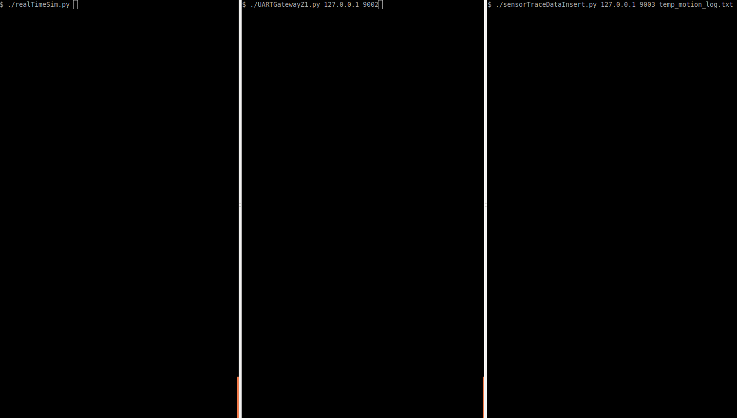
Next, we go to src/support/cape/sim and open 3 shells. In each shell, we set the following Python scripts for the Cape Fox simulation:
-
./realTimeSim.py(to run Cape Fox simulation) -
./UARTGatewayZ1.py 127.0.0.1 9002(to connect to Cape Fox serial port on each simulated mote) -
./sensorTraceDataInsert.py 127.0.0.1 temp_motion_log.txt(to connect to Cape Fox to send sensor measurements from the trace file)
At this moment, the 3 shells should look similarly to the figure below:
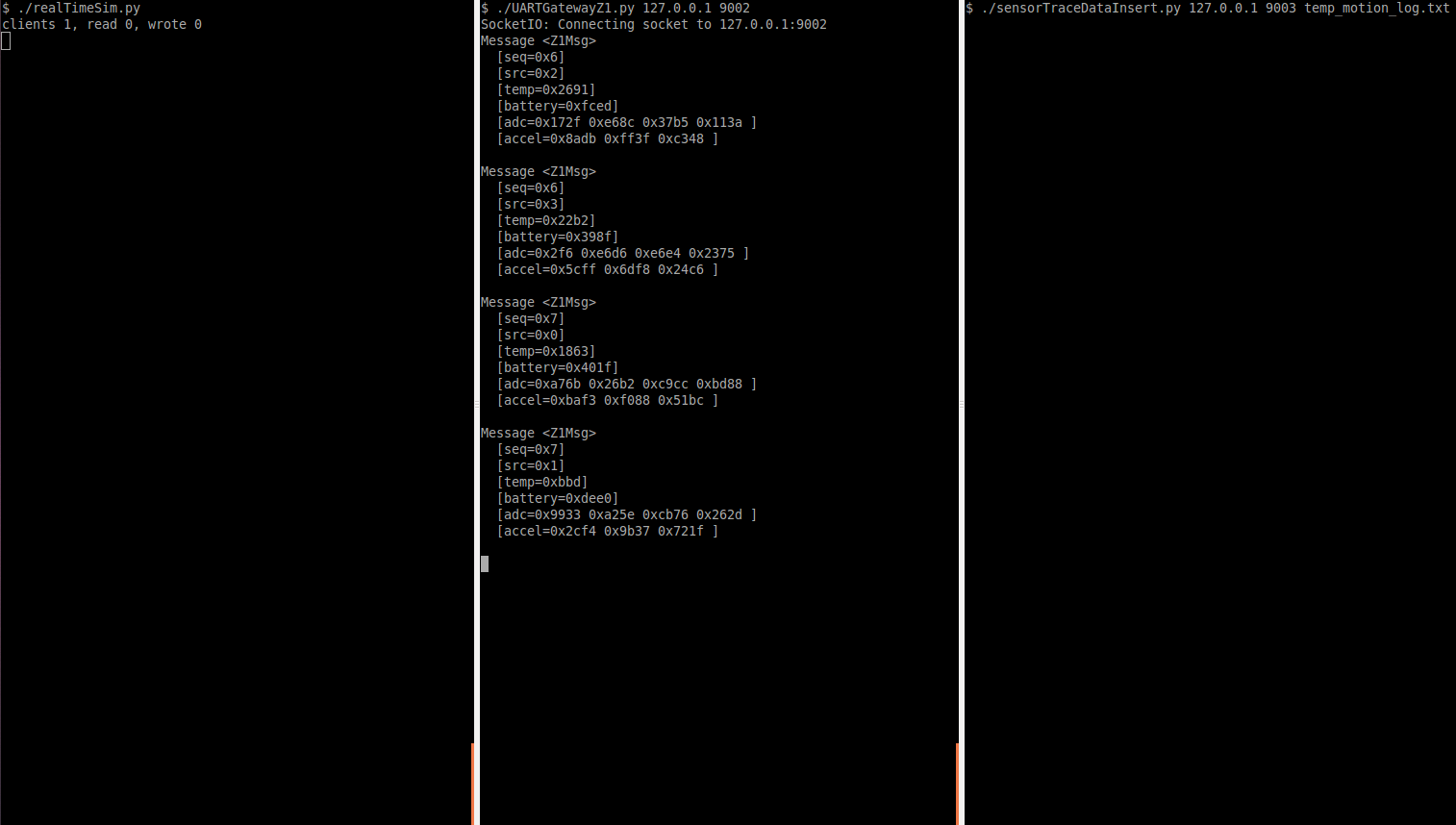
After starting the Cape Fox and connecting to the simulated serial ports, the output should look as follows:
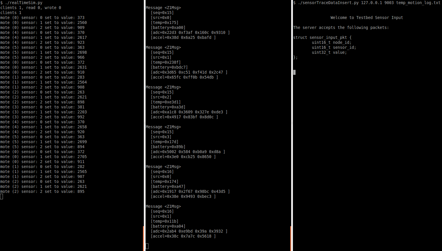
Finally, after starting the script that sends sensor measurements, the shells will looks as follows:
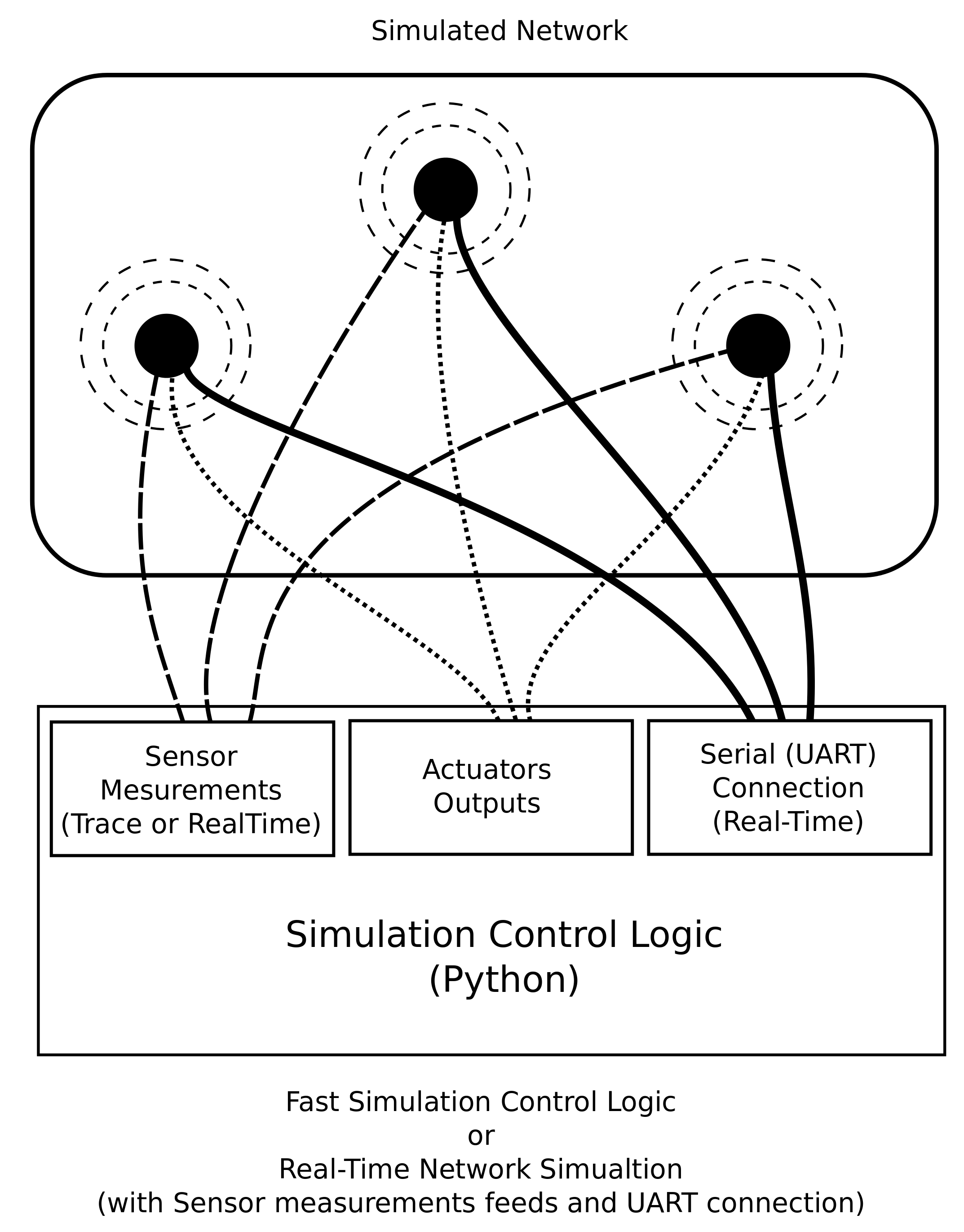
The following figure summarized the Cape Fox architecture:
As mentioned before, when sensor data is not inserted during the simulation, at run-time Cape Fox generates the sensors' measurements by computing the simulatedData function, implemented as follows:
uint32_t simulateData(uint16_t node_id, uint8_t io_id, long long int time_val) {
	return (io_id + 1) * SIN_AMPLITUDE * sin(time_val * (node_id + 1));
}
where SIN_AMPLITUDE is set to 10000, and node_id is the address of the mote, and io_id is the sensor's channel number. The time_val is the current simulation time.
When the sensors measurements are remotely provided, then the Cape Fox simulator stores them in run-time memory. For each simulated mote, Cape Fox creates MAX_SENSOR_INPUTS different channels, simulating sensing of MAX_SENSOR_INPUTS different sensors. By default, MAX_SENSOR_INPUTS is set to 10. Cape Fox also creates MAX_ACTUATOR_OUTPUTS, simulating motes' actuation signals. By default, MAX_ACTUATOR_OUTPUTS is set to 10. The figure below shows the input and output channels for each simulated mote.
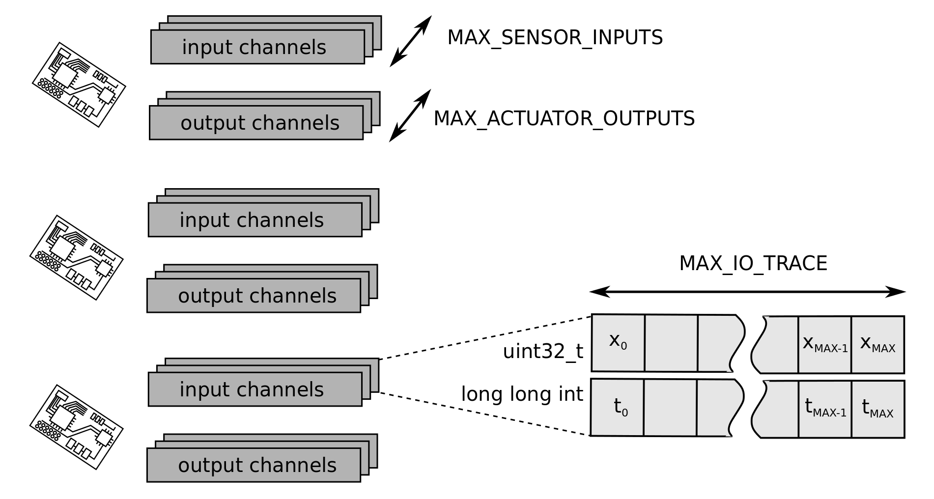
Each simulated input or output channel consists of two arrays: data and timestamp array. The data array stores the input or output value. The timestamp array stores the time when the sensor measurement was inserted or when the actuator signal was generated. At run-time, both arrays can grow dynamically up to the length of MAX_IO_TRACE, which by default is set to 4096.
During simulation, Cape Fox returns the last sensor/actuator value, when the inserted sensor/actuator value is recent with respect to the simulation time. In particular, when the last time when the data was inserted is not older from the current simulation time then the difference between the time stamps of last two I/O entries multiplied by IO_TIME_STEP_ERROR, then the simulator returns the last value. By default, IO_TIME_STEP_ERROR is set to 2.6. So, when
| t[MAX-1] - simulation_time | < IO_TIME_STEP_ERROR * | t[MAX] - t[MAX-1] |
then the returned values is x[MAX], otherwise the simulator assumes that there are no more data entries, and it wraps around the input/output channels to return the past inserted measurements. The index of the value array is found by computing:
( ( t[MAX] - t[0] ) % simulation_time ) * MAX_IO_TRACE / ( t[MAX] - t[0] )