
A daily-frequency backtesting engine for multi-asset equity strategies, built to demonstrate the things that actually matter in quantitative development: correct vectorized computation, explicit handling of look-ahead bias, realistic transaction cost modelling, and honest out-of-sample validation.
The headline finding is a negative one, which is the point: of three classical strategies tested on five years of real US equity data, none beats a passive SPY position on a risk-adjusted basis, and one of them only looks profitable until it is validated out of sample.
docker build -t backtest-engine . && docker run --rm backtest-engineThat single command reproduces every number and chart below. No API keys, no network, no manual steps — the price cache is committed.
BACKTEST.md is the long-form technical writeup: the problem, the architecture and why it is shaped that way, the bias mitigations and how each is tested, full results, and the engine and performance analysis behind them.
476 S&P 500 constituents across all 11 GICS sectors, 2019-01-02 to 2023-12-29 (1,258 trading days), net of 5bp transaction cost and 2bp slippage, positions lagged one day.
The universe is current index membership filtered to names with complete
coverage of the window: 27 of 503 are dropped for listing late (COIN, ABNB,
PLTR, CARR…) or for trading under a symbol that did not exist before 2024.
That filter is reported, not silent — python -m engine.data_loader names
every drop — because it is a selection rule, and it biases the survivors
towards companies already listed in 2019. configs/universe.yaml states what
that costs.
| strategy | ann return | ann vol | Sharpe | Sortino | max DD | Calmar | OOS Sharpe | beta | turnover |
|---|---|---|---|---|---|---|---|---|---|
| mean reversion | −8.03% | 17.83% | −0.38 | −0.52 | −38.2% | −0.21 | −0.20 | 0.39 | 0.206 |
| momentum | 13.57% | 22.26% | 0.68 | 0.95 | −34.0% | 0.40 | 0.77 | 0.87 | 0.160 |
| pairs | 1.55% | 16.33% | 0.18 | 0.26 | −19.4% | 0.08 | −0.18 | 0.10 | 0.014 |
| SPY buy & hold | 15.60% | 20.99% | 0.80 | 1.11 | −33.7% | 0.46 | — | 1.00 | — |
OOS Sharpe is from walk-forward validation: 5 folds of 504 training days
followed by 126 out-of-sample days, with parameters and pair selection made
on training data only.
Momentum loses to SPY on every axis, and the wider universe is what exposed that. On an earlier 40-name universe momentum returned 19.4% against SPY's 15.6% — more money, worse Sharpe, defensible as "a leveraged index fund." Across 476 names it returns 13.57% against the same 15.6%, so it now loses on the raw number too, at higher volatility (22.3% vs 21.0%) and a lower Sharpe (0.68 vs 0.80). Beta 0.87 says most of what it does earn is market exposure anyone can buy for free, and an information ratio of −0.11 says the residual is not out-performance at all. Ranking 40 names is a thin cross-section; ranking 476 is the test the strategy was always claiming to pass.
Pairs trading is the cautionary tale, and widening the search made it a better one. 476 tickers is 113,050 candidate pairs, up from 780. The best one found — HBAN/TFC, two regional banks — cointegrates at p = 0.0007, far more convincingly than anything available in the small universe. Full-sample Sharpe 0.18; walk-forward Sharpe −0.18. That is the entire lesson in one line: searching 145× harder bought a much better-looking pair and no out-of-sample edge. At p < 0.05 over 113,050 tests, roughly 5,600 pairs clear the bar by chance alone, so "it passed a significance test" is nearly uninformative unless the selection happened before the period you score on.
Mean reversion is destroyed by costs, not by being wrong. It trades 478,302 times at an average daily turnover of 0.21 — 3.6% of capital per year in fees alone, before it has been right or wrong about anything. A backtest without a cost model would show something far more flattering, which is precisely why the cost model exists.
Pairs still has the lowest market exposure — beta 0.10 and a −19.4% max drawdown against everyone else's −34% to −38%. But it is much less neutral than the two-name version of this strategy was (beta −0.02, 5.8% vol on the 40-name universe); a spread between two regional banks carries real sector risk, and 2023 charged it for that.

Equity on a log scale so equal percentage moves are equal distances. Shaded bands mark the 2020 COVID crash and the 2022 selloff — every series reacts to both, which is a visual sanity check on the data as much as a narrative.

The flat first stretch is the 126-day lookback warming up, not a data gap. Drawdowns land where they should: −32.3% at COVID, and again through 2022.

A single full-sample Sharpe hides when a strategy worked. At a 60-day window every series swings between roughly −6 and +7, which is worth internalising: short-window Sharpe is extremely noisy, and a strategy "working" for two months means almost nothing.
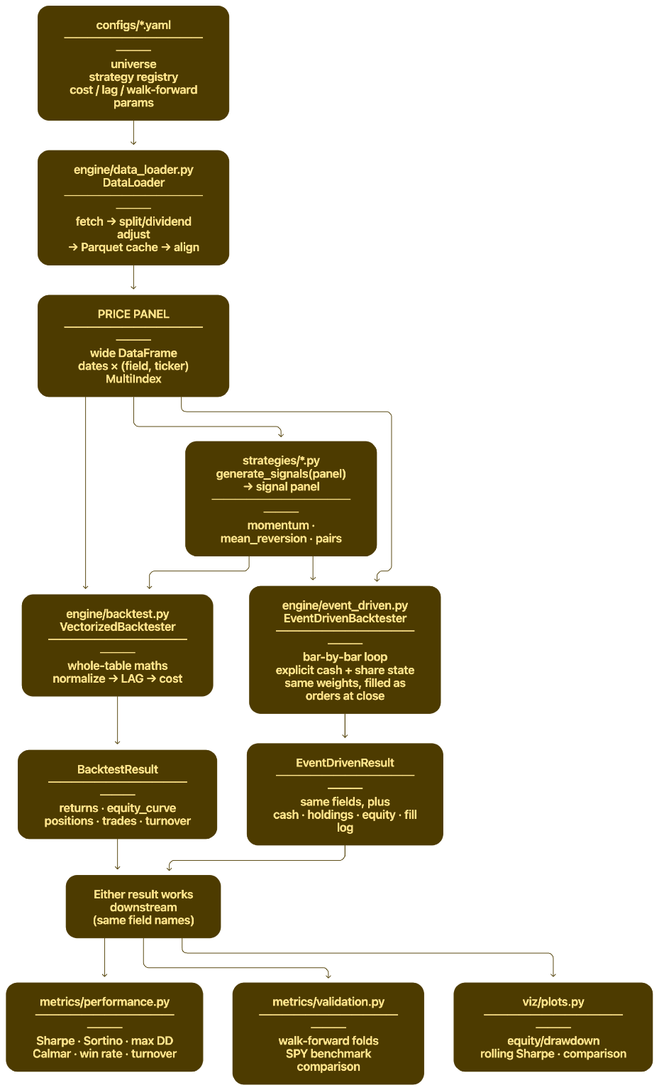
Five design decisions hold the whole thing together:
One panel shape everywhere. Prices and signals are both wide DataFrames
with dates as rows and tickers as columns. Because they are identically
shaped, "what I held times what it returned" is a single element-wise
multiply over the entire history — no loops, no reshaping. An AST check in
the test suite confirms engine/backtest.py contains zero for loops.
One strategy interface. Every strategy implements
generate_signals(price_panel) -> signal_panel. The engine has no idea which
one it is running; adding a fourth means writing one file and one YAML block,
with no engine change.
Configuration is not code. Universe, costs, lag, allocation method and
walk-forward windows live in configs/*.yaml.
Two engines, one allocation step. The event-driven engine calls the
vectorized engine's _target_weights, so the two cannot disagree about what
to hold — every difference in their output is attributable to how it gets
held. That is what makes comparing them informative rather than noisy.
The lag is a single, deliberate, commented line. See below.
A signal computed from day t's closing price cannot be traded on day t — that price does not exist until the market has closed. The engine therefore holds yesterday's target:
return weights.shift(self.lag_days).fillna(0.0) # engine/backtest.pyTo show this is not decorative, here is the same three-day toy dataset run with and without that line:
| total return | |
|---|---|
| lag removed | +20.77% |
| lag present | −0.07% |
A losing strategy becomes a 21% winner from one missing shift(). The engine
refuses to run with lag_days=0 rather than offering it as an option, and
tests/test_backtest.py fails loudly if the lag is ever removed.
Two subtler forms are handled too:
- Volatility-based sizing derives from prices, so it is folded into the weights before the lag — otherwise it would leak through the back door while the signal itself looked correctly lagged.
- Pair selection in
strategies/pairs.pyuses a formation window and never trades inside it. Choosing a pair over the full history and then backtesting on that same history is selection bias, and it is nastier than a missingshift()because every individual day's arithmetic still looks right. The −0.25 out-of-sample Sharpe above is what that costs.
engine/backtest.py computes the whole history in a handful of whole-table
operations. engine/event_driven.py computes the same history by simulating
it — one bar at a time, holding a cash balance and a share count per ticker,
placing orders that get filled at the close.
Building both was not redundancy. It was the only way to find out what the fast one was quietly assuming.
With costs switched off, the two engines produce identical gross returns to floating-point precision (max difference ~1e-15 over 1,258 days). That is the assertion worth caring about: gross return is just "what I held times what it did", with no modelling choices in it. If it diverged, the engines would be disagreeing about the lag or the allocation, which is a bug rather than a difference of opinion.
Getting there required fixing a real off-by-one. Filling at the close of bar
t means the position established today is exposed to tomorrow's move —
the simulation is already one bar lagged, structurally. So lag_days = 1
maps to zero extra delay in the event loop, and the index offset is
t - (lag_days - 1). Writing the obvious t - lag_days double-lags the
entire book: nothing crashes, the equity curve still looks plausible, and the
two engines quietly disagree by one day forever.
test_positions_match_vectorized is what pins this down.
strategy          gross diff  vec return  evt return  vec turnover  evt turnover  cost gap    fills
---------------------------------------------------------------------------------------------------
mean_reversion       1.8e-05     -51.03%     -51.22%        0.2204        0.2251     0.41%   41,527
momentum             5.2e-05     142.38%     140.77%        0.1721        0.1796     0.66%    4,960
pairs                1.2e-05      14.77%      14.19%        0.0127        0.0185     0.51%      956
(python -m engine.run prints this table; gross diff is above 1e-15 here
only because costs are on — see the third bullet below.)
Event-driven turnover is higher for every strategy, and the total return is correspondingly lower. Three distinct mechanisms, in order of how much they matter:
1. Weight drift is a trade the vectorized engine cannot see. The
vectorized engine measures turnover as the change in target weights,
|w[t] − w[t−1]|. Hold a permanently constant signal and that is zero
forever — it charges for the initial buy-in and nothing after. But holding a
constant weight is not holding a constant position: prices move
overnight, the weights drift apart, and pulling them back to target is a real
trade that a real broker really bills for. The event-driven engine tracks
shares, so it sees those trades and charges for them.
This shows up most starkly in pairs, where reported turnover rises 46% (0.0127 → 0.0185). Pairs holds a near-static two-leg position, so almost all of its true trading is drift correction — the exact category the vectorized engine is blind to. The strategy that looked cheapest to trade is the one whose costs were most understated.
2. Cost timing. A trade decided from bar t's close is filled at bar t's close, so the cash leaves at bar t. The vectorized engine charges it against bar t+1, the day the position becomes effective. A one-bar shift in the cost series — immaterial to the total, visible day by day.
3. Orders are sized on pre-commission equity. The commission is not known until the order exists, so the order is sized off current NAV and the fee comes out after. The book is therefore a fraction of a basis point above 100% gross once the fee is paid. This is what a live system does, and it is why gross returns match exactly only at zero cost; with 7bp of costs they agree to ~1e-5.
None of these reverse a conclusion. Momentum still beats the benchmark on return and loses on Sharpe; mean-reversion is still bad; pairs is still a low-volatility, low-return book that fails out of sample. The engines are directionally consistent, which is the checkpoint. What changed is the confidence interval around the cost estimate — and the knowledge that it is biased optimistic in the vectorized engine, by more for low-turnover strategies than high-turnover ones.
| Vectorized | Event-driven | |
|---|---|---|
| Unit of thought | weights | shares and cash |
| Speed (476 tickers × 5y) | ~16–25 ms | ~15–25 ms (C++), ~40–270 ms (Python) |
| Can express whole-share orders | no | yes |
| Can express a no-trade band | no | yes |
| Sees weight drift | no | yes |
| Tracks cash | no | yes |
| Could place a live order | no | yes |
The event-driven engine adds two frictions the vectorized one cannot represent at all, both off by default and both tested:
fractional_shares: false— whole-share orders only. A fixed rounding error in dollars, so it dilutes as the account grows;test_whole_share_error_shrinks_with_capitaldemonstrates exactly that.rebalance_threshold— a no-trade band that skips orders below a given fraction of equity. The standard fix for drift-driven churn: it cuts turnover and cost at the price of letting weights wander from target.
Why real trading systems are event-driven. Not for accuracy — for identity. In production the backtest and the live trader must be the same code path, and a live trader is inherently an event loop: a bar arrives, state updates, orders go out. A vectorized backtest cannot be run live at all; it needs the whole future in a DataFrame before it can compute anything. It is the right tool for research throughput, and it will lie to you about execution, quietly and in the optimistic direction.
The event-driven bar loop is ported to C++ in cpp/event_loop.cpp and bound
with pybind11. It is a line-for-line translation of _simulate_python —
same variable names, same order of operations — because the point is to
measure the language, not to compare two different algorithms.
The extension is optional. Without a compiler the engine falls back to
the Python loop and every number in this repo is unchanged; only the runtime
differs. python -m engine.run prints which backend it used.
python setup.py build_ext --inplace   # builds engine/_fastloop.*.so
python scripts/benchmark_cpp.py # correctness, then wall clockThe tempting target is the vectorized engine's returns aggregation. Porting it would have been a waste: it is already NumPy, which is already compiled C with SIMD, so the honest measurement would have been about 1x.
The event-driven loop is the opposite case. It is irreducibly serial — bar t+1's equity depends on bar t's fills — and in Python each bar pays for roughly fifteen separate NumPy calls. The per-call cost (allocate a temporary, check dtypes, refcount, return) is fixed, so how much of it there is to remove depends entirely on how much real arithmetic sits underneath — which is to say, on how wide the book is.
So Phase 6 was not decoration in front of Phase 7. It is what made a real speedup possible to measure at all.
Correctness first — a speedup from code that computes something else is not a speedup. Across all three strategies on the real panel, the largest disagreement in daily returns is 6.9e-14, with identical fill counts. That is float-ordering noise: NumPy reduces pairwise, the C++ loop accumulates in order, so they differ in the last bit.
WALL CLOCK  (real panel: 1,258 bars x 476 tickers)

strategy              python       cpp   speedup     (full run() end to end)
----------------------------------------------------------------------------
mean_reversion      248.42ms    9.93ms     25.0x         269.8ms ->   27.9ms  (9.7x)
momentum             39.36ms    4.62ms      8.5x          52.2ms ->   16.3ms  (3.2x)
pairs                11.13ms    3.90ms      2.9x          26.4ms ->   17.6ms  (1.5x)
Two numbers, on purpose. The loop is what was ported, so ~3–25x measures
the port. But a user calls run(), which also builds a dozen pandas objects
around the loop — constant work C++ never touches — so the end-to-end gain is
1.5–10x. Quoting only the first would overstate what anyone experiences.
(Run-to-run variance across strategies is real; scripts/benchmark_cpp.py
regenerates the table.)
These numbers are much lower than they were, and that is the interesting part. On the earlier 40-name universe the same table read 28–47x on the loop and 5–10x end to end. Widening the book to 476 tickers cut the advantage by roughly a factor of three without a line of either implementation changing — exactly what the scaling table below had predicted, which is the nicest kind of confirmation: a mechanism argued from a synthetic sweep, then paid out on the real workload.
Holding bars fixed and varying only the width of the book shows the mechanism directly:
SCALING  (1,258 bars, varying width -- synthetic)

  assets      python       cpp   speedup   python us/bar   cpp us/bar
---------------------------------------------------------------------
       5      9.65ms    0.06ms    161.8x            7.67         0.05
      20     17.38ms    0.38ms     45.6x           13.81         0.30
      40     28.94ms    0.70ms     41.5x           23.01         0.55
     100     61.23ms    1.91ms     32.0x           48.67         1.52
     500    316.08ms   11.94ms     26.5x          251.26         9.49
The Python loop pays the same fixed dispatch cost per NumPy call whether the arrays hold 5 elements or 500, so the narrower the book, the more of the runtime is pure interpreter tax — and the more there is to remove. Read the two columns on the right: from 5 to 500 assets the Python loop gets 33× slower per bar while the C++ loop gets 190× slower, because C++ was only ever paying for the arithmetic and the arithmetic is what grew.
That is why the real-panel numbers fell when the universe did not change shape but did change size, and it is the honest ceiling on this kind of port: the wider the book, the less of the runtime is interpreter tax and the less there is for C++ to win back.
The claim is therefore not "C++ beats NumPy at arithmetic." It is "C++ does not pay a dispatch tax fifteen times per bar." That distinction is the whole result.
Two things had to change, and both were improvements:
The fill criterion. The original loop counted an order as real when the
share delta exceeded an absolute 1e-12. That is not scale-free — 1e-12
shares of a $1 stock and of a $1000 stock are not the same event — and it
broke the port. Hold one asset at 100% and the target share count is exactly
what you already own, so every bar's delta is float dust sitting right on the
threshold, tipping either way depending on summation order. The two backends
disagreed on the fill count by one. Measuring the order as a fraction of
equity puts that dust at ~1e-15, three orders of magnitude clear of the
line, and makes the criterion stable across implementations.
Tolerances that respect cancellation. Cash is a residual: equity minus everything held. In a long/short book those are two ~$2M numbers that nearly cancel to a balance of a few dollars, so it keeps absolute precision at the scale of the inputs while its relative precision is destroyed. The tests compare money in dollars and ratios relatively; one tolerance for both would either fail on cash or wave through a real divergence in the returns.
The loop also releases the GIL, so two backtests can run on two threads.
test_cpp_backend_releases_the_gil asserts that by timing it — otherwise
removing the release would break nothing any other test could see.
docker build -t backtest-engine .
docker run --rm backtest-engine
To keep the generated charts:
docker run --rm -v "$PWD/notebooks/results:/app/notebooks/results" backtest-enginepython3 -m venv .venv && source .venv/bin/activate
pip install -r requirements.txt
python -m engine.run # full pipeline: table + charts
pytest -q # 106 tests
python scripts/make_charts.py # charts only
pip install -r requirements-dev.txt
ruff check . # what CI lints withCI runs the same commands on Python 3.11/3.12/3.13, builds the C++ extension so the backend-equivalence tests actually run, and separately builds and runs the Docker image.
Optionally build the C++ bar loop. Everything runs without it — the engine falls back to the Python loop and the results are identical — but it makes the event-driven engine 5–10x faster end to end:
python setup.py build_ext --inplace   # needs a C++17 compiler
python scripts/benchmark_cpp.py       # verifies equivalence, then times it
The Docker image builds it, so docker run always takes the fast path.
The per-ticker Parquet cache is committed, so this is not normally needed. Yahoo blocks scripted HTTP clients (429 on every network tested, with or without cookies or the crumb handshake) while still serving browsers, so the fetch runs from a browser console:
- open https://finance.yahoo.com
- paste
scripts/yahoo_browser_fetch.jsinto the JavaScript console mkdir -p data/browser && mv ~/Downloads/yahoo_panel_*.json data/browser/python -c "from engine.data_loader import DataLoader; DataLoader().ingest_browser_panel('data/browser')"
Stated plainly, because a backtest that does not list these is hiding them.
- Survivorship bias, and it got worse with size. The universe is current S&P 500 membership, so firms that went bankrupt, were acquired, or shrank out of the index over 2019–2023 are absent entirely, and 118 of the 503 names joined the index after 2019-01-01 — holding them from the start is a bet nobody could have placed. The full-coverage filter then removes 27 more for listing late, which biases the survivors further towards already-established companies. Every one of those errors flatters results, including the SPY benchmark. A point-in-time membership file is the only real fix and this project does not have one.
- Daily data only. No intraday prices, no order book, no microstructure. Fills are assumed at the adjusted close.
- Costs are a flat basis-point model. Real costs vary with size, liquidity and urgency, and market impact grows with position size. A strategy trading size would face worse fills than 7bp.
- No borrow costs or shorting constraints. Short positions are assumed freely available and free to hold. Neither is true, especially for the names a mean-reversion strategy wants to short.
- No risk-free rate. Sharpe and Sortino use a 0% hurdle. Over 2019–2023, rates went from ~2.4% to ~5%, so real risk-adjusted numbers are worse than those shown.
- Pairs re-selection is fixed per fold, not rolling. Within a fold, the pair is chosen once from the formation window. A production system would re-select continuously.
- Five years is a short sample. It contains one crash and one bear market. Five folds of walk-forward is enough to catch gross overfitting, not enough for statistical confidence.
- A backtest is not live performance. No slippage from latency, no partial fills, no exchange outages, no risk limits, no capital constraints.
configs/     universe, strategy registry, backtest parameters (YAML)
data/cache/  committed per-ticker Parquet price cache
engine/      data_loader.py · backtest.py · event_driven.py · run.py
strategies/  base.py · momentum.py · mean_reversion.py · pairs.py
metrics/     performance.py · validation.py
viz/         plots.py
cpp/         event_loop.cpp (optional pybind11 extension)
scripts/     yahoo_browser_fetch.js · make_charts.py · benchmark_cpp.py
tests/       106 tests
.github/     CI: lint, tests on 3.11-3.13, Docker build
notebooks/results/   generated charts and results table
MIT — see LICENSE.