SVM using Numpy

---

Support Vector Machine is used for finding an optimal hyperplane that maximizes margin between classes. SVM’s are most commonly used for classification problem. They can also be used for regression, outlier detection and clustering. SVM works great for a small data sets.

There are two classes in the below example. One is denoted by ‘- ‘and other by ‘+’. Both the classes are plotted on a 2D graph and separated using randomly guessed hyperplane. Using SVM, a decision boundary can be drawn that can best separates two classes. This decision boundary is called as a hyperplane. Hyperplane is a linear decision surface. For 2-dimensional space, hyperplane will be (2–1) 1 dimension. Similarly, for a three-dimensional space, hyperplane will be (3–1) 2-dimensional

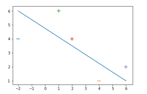
A discriminative classifier can be created using support vector machines. Decision boundary is drawn by maximizing the margin(space) between the line(hyperplane) and classes. Points that are closest to the decision boundary are called support. They are called so because they support the creation of the hyperplane.

Goal is to find the function that best represents the relationship between the variable. Weights are updated through optimization technique and gradient descent is the one used here. Optimization is nothing but minimizing the loss or an error function.

Loss

Hinge loss is a very popular loss function for SVM

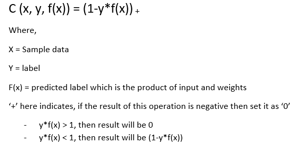
Objective is to minimize the following function Here, first term is the regularizer and second term is the hinge loss calculated for all the data points. Gradient descent is done by taking partial derivative of both terms.

Code

Imports

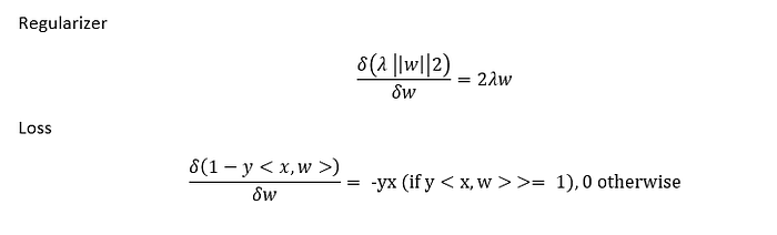
We use only:

• numpy - for creating model
• matplotlib - for making graphs
• accuracy_score - for see how model do its best

import numpy as np
from matplotlib import pyplot as plt
from sklearn.metrics import accuracy_score

Making SVM with one function

def svm_function(x,y):
    #weight
    w = np.zeros(len(x[0]))
    
    #learning rate
    l_rate = 1
    
    #epoch
    epoch = 10000
    
    #output lists
    out = []
    preds = []
    
    #training svm
    for e in range(epoch):
        for i, val in enumerate(x):
            val1 = np.dot(x[i], w)
            if (y[i]*val1 < 1):
                w = w + l_rate * ((y[i]*x[i]) - (2*(1/epoch)*w))
            else:
                w = w + l_rate * (-2*(1/epoch)*w)
    
    for i, val in enumerate(x):
        out.append(np.dot(x[i], w))
    for i in out:
        if i < 0:
            preds.append(-1)
        else:
            preds.append(1)
    
    return w, preds

let's see how it works

print('Calculated weights')
print(w)

output:
Calculated weights
[ 1.62876617  3.23017165 11.37623851]

And finally let's see our prediction

print('predicted output')
print(out)

predicted output
[-1, -1, 1, 1, 1]

Accuracy

Fortunately accuracy is 1.0

print('accuracy:', accuracy_score(out, y))

accuracy: 1.0

That's all