Domain Image Showcase

Domain -- The image showcase (two public datasets larger than RAM)

Notebook: 35_archive_showcase. The legs run from the command line, python -m dtfit_experimental.study.showcase.cli; the notebook reads the tables they write and reruns a sample of stations when the archives are on disk.

Intent

Measure the image core's three claims on public data against published results, on a workstation and on a Raspberry Pi 5: a fit from the image equals the fit from the raw samples; the image is additive, so a dataset larger than RAM reduces in one pass and across machines; and the analysis moves to the weak machine.

Methods under test (dtfit)

• ImageStream accumulator -- one pass per station file, fixed memory, the whole-span image per component.
• ImageStream block mode -- yearly (NGL) and daily (NOAA) block images with detect="previous" drift flags, assembled with assemble.
• channel form -- all stations sharing a day's hourly grid projected in one GEMM, on numpy and on the cupy backend, swept over the batch width.
• dtfit.image.fit from a stored image -- the batch fit the Pi runs on what it received. The order comes from the span-and-density rule (max(16, ceil(8 * span) + 16), capped at n - 2 and n / 4); dtfit.image.coverage is recorded per station beside it and marks the rows where that order cannot represent the model.
• ImageFilter(basis="legendre") -- the streaming tracker and its DriftDetector, in a detection configuration and a tracking configuration.
• the image and the samples on the wire -- a length-prefixed JSON header and a float64 payload: block images from the Pi to the PC, raw samples from the PC to the Pi with block images coming back.

Baseline methods (published, not ours)

• numpy.linalg.lstsq on the same rows -- the exactness reference; the models are linear, so this is the analytic answer.
• MIDAS velocities (Blewitt, Kreemer, Hammond, Gazeaux 2016) -- the published robust trend per NGL station, with its uncertainty.
• the NGL step database -- 142,474 dated equipment changes and earthquake steps, with magnitude and epicentral distance.
• NOAA 1991-2020 hourly normals -- the published climatology for 465 US stations.

Data

dataset	files	rows	size	model
NGL daily positions (tenv3)	23,769 stations (23,175 reduced, 594 failed)	about 83.3 million	17.0 GB	c + v t + a1 cos(2 pi t) + b1 sin(2 pi t) + a2 cos(4 pi t) + b2 sin(4 pi t) per component
NOAA Global Hourly 2024	13,345 station-years (12,677 reduced, 668 failed)	about 116 million	51.6 GB	annual and semiannual on a trend (order 24); the diurnal cycle from one-day images (order 16)

1. The fit from the image equals the fit from the samples

Worst relative parameter difference against lstsq on the same rows, per station and component (ngl_exact.csv, isd_exact.csv); the gate is 1e-8 and the score is purely relative on every parameter. The NGL reader subtracts the first row's integer metre column and carries it as metadata: with the absolute coordinate in place (5,361,769 m on ALBH north) the score would read 3e-15 while the velocity and the cycle amplitudes miss 1e-5 relative.

dataset	fits	worst (any gate)	median (ok/FAIL)	over the 1e-8 gate	ill-conditioned	undersampled
NGL	69,525	1135.29	2.90e-13	2,782	1,275	1,542
NOAA station-year	12,677	1.06	1.65e-13	937	835	131
NOAA day images	3,367	2.09e-11	--	0	--	--

"Over the 1e-8 gate" is every row scoring above the gate whatever its excuse; it is larger than the ill-conditioned count because 1,507 NGL and 102 NOAA rows are both UNDERSAMPLED and over the gate, counted in "undersampled" and not repeated here. The NGL worst, 1135.29, is one such UNDERSAMPLED row. The median column is dropped for the day-images row: the 3,367 day scores are stored one station-year maximum at a time (isd_exact_days.csv, 465 rows), so the only median available there (3.87e-13) is the median of those 465 maxima, not of the 3,367 day scores, and reads high for it. The 2.09e-11 worst is also the worst of those 465 maxima; the day-image scores that isd_exact.csv carries inline for all 6,797 checked station-years reach a worse 2.17e-11. The day-images row is a different statistic from the other two: it checks the day sub-image against its own raw hourly rows (day_score) rather than the whole-station-year fit, so its count is checked days, not station-years.

A miss inside the attainable bound (design_cond**2 * (coverage + EPS * gram_cond)) is not a pass, only an unfalsifiable row: for the 1,275 NGL ILL-CONDITIONED rows the bound has a median of 2.95e+04 and exceeds 1 (a 100 percent relative miss permitted) on 1,156 of them; for the 835 NOAA rows the bound has a median of 3.40e+10 and exceeds 1 on all 835. The median ratio of bound to actual score is 1.5e+11 (NGL) and 5.9e+16 (NOAA), so on those rows the verdict says only that the raw solve is itself undetermined at that order and density, not that the image agrees with it.

The Legendre order is max(16, ceil(8 * span_years) + 16) for NGL, capped at n - 2 and at n / 4, and 24 for a NOAA station-year: eight coefficients per year alone leaves 2.3e-3 at a three-year span and 5.2e-7 at eleven years, and the additive margin is what carries the short spans through the gate. The density cap is what keeps a sparse station representable; the stations it cannot save are reported as UNDERSAMPLED from their coverage value and counted separately, not as failures. That is 2.2 percent of NGL stations.

G is a deterministic function of the grid, the basis and the order, so a receiver could rebuild it instead of receiving it: the worst rebuild error over the whole set is 1.24e-16, at rounding but not bit identical, which is why the run ships G (leg 5's bit-exactness check needs the accumulated one).

2. The reduction: throughput, memory, size

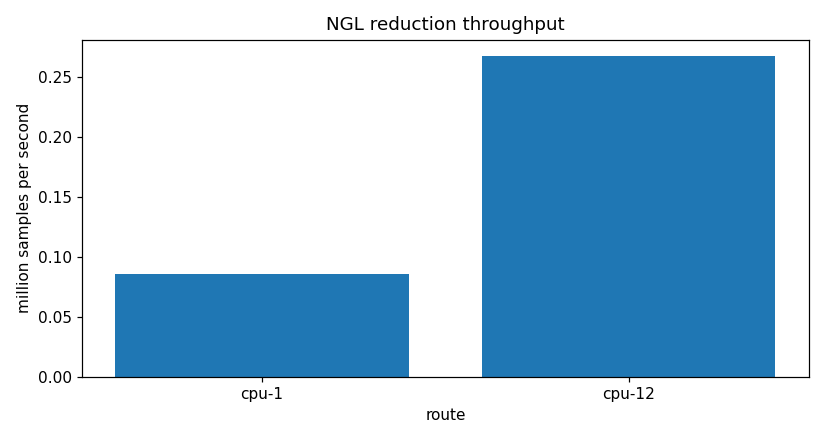
From throughput.csv, throughput_n4000.csv and ngl_reduce.csv / isd_reduce.csv.

route	samples/s	traced peak	resident peak	note
raw disk read	--	--	--	3527.67 MB/s (page-cache speed; the files were just read by this session, not a cold drive)
one process	85,566.2	48.86 MiB	674.53 MiB
12 processes	267,553.6	0.23 MiB	747.29 MiB	traced covers the parent only
float32 accumulation	--	--	--	2.09e-08 rel error against 0.00e+00 float64

The memory claim is stated against the resident set, not the traced allocation: tracemalloc does not follow a process pool's children, so a pooled traced peak means nothing. The gate is the one-process resident peak on 200 stations against the same on 2,000: 674.53 MiB against 671.79 MiB, which is met, but the resident number is dominated by a flat baseline, not by any one station: a fresh interpreter that only imports the reducer already sits at 197.6 MiB, and a spawned child reducing 40 synthetic 4,000-row stations peaks at 579.2 MiB resident against an 8.9 MiB traced peak -- it is the traced peak, not the resident one, that actually tracks the largest station's own grid and coefficients.

dataset	raw	arrays (S + G + grid)	ratio	stored (.npz)	ratio	S	G	grid
NGL	17.0 GB	18.402 GB	1.08x raw	14.41 GB	0.85x raw	191.8 MB	12939.1 MB	5270.7 MB
NOAA 2024	51.6 GB	0.996 GB	0.02x raw	0.29 GB	180x smaller	2.5 MB	63.4 MB	930.1 MB

Two different numbers, both real: "arrays" is S, G and grid at their in-memory dtype, the quantity a receiver holds after unpacking; "stored" is the .npz file the reducer actually writes, which repacks and compresses each array. They diverge because compression works on G and grid very differently, so the two columns are never expected to agree, and no other column in this table is their sum.

The two datasets say opposite things and the report says both. For NOAA the order is fixed at 24 while the raw file grows with the reporting rate, so the stored .npz files are about 180x smaller than the raw bytes, and the uncompressed arrays alone already come to only 0.02x raw. For NGL the order follows the span, so G grows as the span squared while the raw file grows as the span: the uncompressed arrays come to 1.08x the raw bytes, and only after compression does the stored tree fall to 0.85x raw, with 19 percent of stations still producing a .npz file larger than their own raw file. The image is a reduction for NGL only in what it lets the receiver do without the samples, and only once compressed -- not in the uncompressed arrays' own bytes.

The GPU row

From gemm.csv: the channel form projects every station that filled a day's 24 hour bins in one Phi^T Y, swept over 500 / 5,000 / all qualifying stations crossed with 1 / 7 / 30 days concatenated into one batch. The row below is the widest point of that sweep, all 13,345 station files at 30 days.

backend	channels	elements/s	gather	note
numpy	94,375	238,727,629.7	535.842s
cupy	94,375	146,814,818.5	535.842s

Phi is 24 by 17, so the arithmetic intensity is low and the Gram update stays on the host whatever the backend: only S is accelerated. The shape of the curve against the batch width is the result. The spec's leg 1 asks for this rate reported next to the disk read rate so an I/O-bound result reads as such; that comparison exists for the CPU rows in throughput.csv only, not here -- gemm.csv is a projection-only sweep with the gather time as its own column (8 to 536 seconds against 0.0001 to 0.015 seconds of projection), so no GPU row sits next to a disk rate.

3. Velocities against MIDAS

From ngl_fits.csv: the whole-span fit and the epoch-weighted mean of the fits between database steps, against the published velocity and its uncertainty.

fit	components	median |z|	within one sigma
whole span	64,722	0.658	61.6 percent
between steps	31,983	0.564	67.7 percent

One image, several models

From ngl_rank.csv: the catalogue (trend, trend_annual, trend_annual_semi, trend_quad_annual_semi) ranked by the image BIC against the ranking from numpy.linalg.lstsq on each model's own design matrix on the raw samples. The two arms share no code, so the agreement below is a measurement.

comparison	model-component fits	same rank	top model agrees (600 components)
image against raw samples	2,400	2,383 (99.3%)	595
Pi against PC, image arm	2,400	2,389 (99.5%)	--

4. Steps and the streaming filter

From filters_ngl.csv and filters_ngl_steps.csv. The detector tests once per window, so the 60-day rule applies to the detection configuration (a trend on a fixed 40-sample window, chosen because 60 samples span more than 60 days once the missing days are counted); the tracking configuration (the full model on 1000 samples) carries the velocity.

Two things the raw recall number would hide, both stated here. First, the denominator: the detector is blind for (warmup + 1) * window samples after each flag and for (warmup + 2) * window - 2 samples at the start (min_window plays no part), and 63.8 percent of consecutive database steps sit closer than one blind period, so recall is reported over the reachable subset with the excluded count beside it. Second, the null: over the 200 stations with a median 9 steps and a median 18.9-year span, the union of the +/- 60-day event windows already covers a median 15.2 percent of the timeline (mean 16.2 percent, up to 58.7 percent on the busiest station), so the observed false-alarm rate is printed next to the rate a randomly placed flag would produce.

configuration	window	cost per update (mean)	steps	reachable	recall (reachable)	median delay	false alarms per station-year (median)	chance rate (median)
detection (trend)	40 samples, fixed	128.0 us	7,179	6,444	4.3 percent	21.0 days	0.066	0.088
tracking (full model)	1000 samples, fixed	402.5 us	7,179	1,342	0.1 percent	44.0 days	0.000	0.000

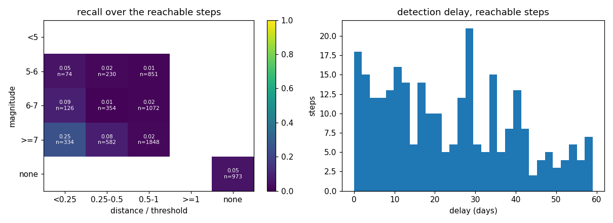
Recall over the reachable steps, binned jointly on magnitude and on distance / threshold (the database's own proxy for whether an offset is expected: 34.6 percent of its earthquake entries are magnitude 7 or above and most of those are far away), with the delay distribution beside it:

The NOAA filter's flags

From filters_isd.csv and filters_isd_flags.csv. An event here is a quality-failed row or a coordinate change, not a step, and an explained flag is not a detection, so the counts are named for what they are.

station-years	flags	explained within two days	events	explanation windows cover (median)
200	2,270	13.6 percent	26,344	5 percent of the year

NOAA annual amplitudes over the whole year

From isd_year_fits.csv: every 2024 station-year fitted from its image alone.

station-years	annual amplitude (median)	10th to 90th percentile	peak day (median)	semiannual amplitude (median)
12,677	9.78 C	2.28 to 17.25 C	195.6	1.45 C

5. NOAA against the published normals

From isd_normals.csv. Both sides of the diurnal comparison are the same statistic: the maximum minus the minimum of the day's reconstruction over the 24 hourly positions, not twice a first-harmonic amplitude (a real day is not a sinusoid and its range exceeds twice the first harmonic by 10 to 25 percent). The normals' 365-day climatology is mapped through 2024's calendar, so no phase difference comes from the leap day.

quantity	stations	median difference (image minus normals)
annual amplitude	465	-0.82 C
annual phase	465	-3.18 days signed (4.09 days median absolute)
diurnal range, monthly medians	465	+1.6 C (+1.73 C per row)

6. The analysis on the Pi

From ngl_fits_pi4000.csv, isd_year_fits_pi.csv, ngl_rank_pi.csv and the *_timing*.csv files each run writes. The Pi holds the images and never the raw files: ngl-rank runs with --no-raw, so the ranking on the Pi reads no station file either.

machine	cores	workers used	RAM	fits	wall time	worst velocity difference
Ryzen 9 9950X3D	16	12	54 GiB	230,751	740.7 s	--
Raspberry Pi 5	4	4	8 GB	32,307	6893.0 s	1.32e-05 m/yr

The worker counts are not the core counts: the PC ran with 12 workers against its 16 cores and the Pi with 4 against its 4, so about 3x of every wall-time ratio below is process count, not machine.

The two rows above are not the same run: ngl-fits ran on the PC's full 230,751 rows and on the Pi's 32,307-row sample, so their wall times are not a like-for-like ratio. The comparable pairs, same command and same row count on both machines, are isd-fits (12,677 rows, 16.8 s against 294.6 s, 17.5x) and ngl-rank (2,400 rows, 28.7 s against 1756.7 s, 61.2x); on ngl-fits itself the per-fit time is 0.0032 s on the PC against 0.213 s on the Pi, about 66x.

The figure below is the leg-1 comparison, not this one: it is the reduction of raw station files on both machines (throughput.csv and throughput_pi.csv), the one place the Pi does touch raw files, run so that the same measurement exists on both hosts.

7. The stream between the machines

From leg5_stream.csv and leg5_groups.csv. The consumer assembles each station's blocks, fits a trend on the assembly and tallies the drift flags the producer's stream raised, so what crosses the wire is checked as analysis and not only as bytes. The trend rather than the full model because assemble cannot raise the order above the blocks' own 12: what a stream of yearly block images supports is a velocity. Latency is the producer's acknowledged round trip per block; the two machines' clock difference is recorded as a diagnostic and never quoted as a latency.

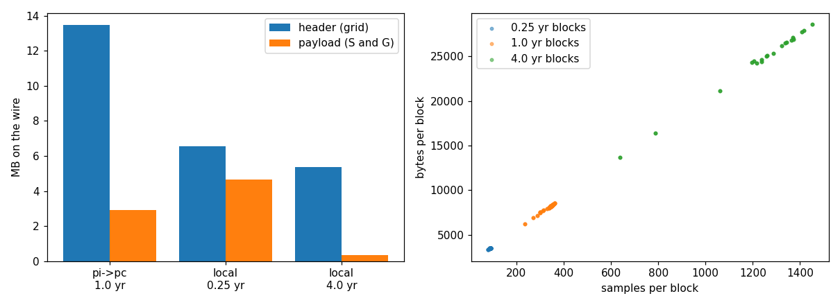
Both directions were measured. The overnight run could not complete the PC-to-Pi direction (its outbound connection to the Pi was refused before the send); on re-measurement the direct connection succeeded and both directions completed, so that refusal was transient. The header cost was also cut: an explicit grid's sample positions now travel in the binary payload rather than the JSON header, which drops the header from about 13 MB to under 1 MB on a run of yearly blocks and the whole exchange from 16 MB to 9 MB.

direction	block length	images	header	payload	images/s	round trip (median)	assemblies mismatched
Pi to PC	1.0 yr	2,000	0.82 MB	8.42 MB	23.4	42.0 ms	0
PC to Pi	1.0 yr	2,000	0.82 MB	8.42 MB	22.4	44.0 ms	0
local	0.25 yr	3,210	1.31 MB	6.96 MB	22.5	--	0
local	4.0 yr	228	0.09 MB	2.62 MB	22.4	--	0

The PC-to-Pi row assembles on the Pi's ARM CPU rather than the PC's x86, so the assembled coefficients round differently in the last bit and the byte-exact digest differs on all 141 groups; the fitted velocity and offset still agree with the PC's own assembly to a median of 2e-15 relative, so the mismatch is architecture rounding, not a transport error. The figure below reflects the earlier header-heavy protocol and is regenerated in the documentation pass.

The other direction: the PC replays, the Pi tracks

From leg5_replay.csv and leg5_track_*.csv: raw samples at a requested rate, the Pi filtering them one at a time with ImageFilter(basis="legendre") and sending its block images back over the same socket. The sustained rate is the largest requested rate at which neither side drops a chunk, and flags_match says whether the flags the Pi raised over the wire are the flags the same filter raised locally on the same 20 stations.

The Pi filters one sample in about 370 microseconds, so it saturates near 2,700 samples per second, and that ceiling shapes the sweep.

requested rate	achieved	dropped	flags	samples tracked
1,000/s	999.6/s	0	22	95,388
10,000/s	2,677/s	3	16	80,892
100,000/s	2,703/s	5	11	67,219
unbounded	2,670/s	0	22	95,388

Below the ceiling the Pi keeps up losslessly and raises the same 22 flags it raises in batch. A fixed rate above the ceiling is the wrong way to push it: the replayer schedules sends at the requested rate, falls behind when the Pi cannot drain them, and drops the chunks it cannot send on time, so samples and the flags that depend on them are lost. The unbounded request has no schedule to fall behind, so the socket's own flow control paces the replayer to exactly the Pi's rate: it lands at the same 2,700 per second but with zero drops and all 22 flags. The lesson is that back-pressure, not a fixed high rate, is how a fast source feeds a slower recursive consumer without loss.

requested	achieved	dropped (sender / receiver)	per-sample cost on the Pi	blocks back	flags match
1,000/s (SSH tunnel)	999.6	0 / 0	399.8 us	280	yes

What this domain says

The exactness claim holds where it applies: the median relative miss against lstsq sits at rounding (2.9e-13 NGL, 1.6e-13 NOAA), and nothing is gated FAIL outright. That is not the same as everything scoring under 1e-8: 2,782 NGL and 937 NOAA fits score above the gate once the excused gates are counted -- 1,275 NGL and 835 NOAA station-years are ILL-CONDITIONED within their own attainable bound, and that bound exceeds one (permits any miss at all) on 1,156 of the 1,275 NGL rows and on all 835 NOAA rows, so for those the verdict says only that the raw solve is undetermined, not that the image agrees with it. 1,507 NGL and 102 NOAA are UNDERSAMPLED and also over the gate (2.2 percent of NGL and 1.0 percent of NOAA fits are UNDERSAMPLED in total). The worst score anywhere is 1135.29, on one UNDERSAMPLED NGL station-component, a reminder that "explained" is not "small": the image agrees with the raw fit only as well as the model's own conditioning and density allow on that station's sampling.

The reduction is flat in memory (674.53 MiB one-process resident peak on 200 stations against 671.79 MiB on 2,000) but not uniformly smaller in bytes: NOAA's fixed order-24 .npz tree is about 180x smaller than its raw files, while NGL's order grows with span, so its .npz tree comes to only 0.85x the raw bytes, and 19 percent of NGL stations still produce a .npz file larger than their own raw file -- the header cost of an irregular grid, which the explicit grid column alone runs to 5.27 GB across the NGL tree. The uncompressed arrays behind that tree are a different, larger number (1.08x raw for NGL, 0.02x raw for NOAA); the two never sum to each other and are not the same claim. The GPU row is not skipped, it is lost to the CPU at every width measured (up to 94,375 channels): with a 24x17 Phi the Gram update stays host-side, so only S is accelerated, and the rate does not rise with the width on either backend, so the product itself is never the cost at this shape.

Against MIDAS the whole-span fit lands at a median |z| of 0.66 with 61.6 percent within one sigma, and splitting on the database's own steps narrows that slightly (0.56, 67.7 percent) -- consistent agreement, not a better fit, since the two arms use the same samples. Ranking four models by image BIC agrees with the raw-sample ranking on 2,383 of 2,400 model-component fits (99.3 percent) and picks the same top model on 595 of 600 station-components; the same comparison run again on the Pi from its own image arm agrees with the PC on 2,389 of 2,400.

The streaming filter is the domain's clearest negative: recall over the reachable steps is 4.3 percent for the detection configuration and 0.1 percent for tracking, and the steps it does catch arrive with a median delay of 21 and 44 days respectively -- the fixed-window stride is a poor match for equipment and earthquake steps on this database, whatever the false-alarm rate (median 0.066 and 0.000 per station-year, both at or below the chance rate a randomly placed flag would produce). On NOAA, 13.6 percent of the diurnal filter's flags are explained within two days by a quality failure or coordinate change, out of 26,344 events whose +/-2-day windows cover a median 5 percent of the year: most flags are unexplained noise, not detected events. The annual-cycle fit from the image alone reproduces NOAA's published normals to a median -0.82 C in amplitude (the image's swing runs smaller) and -3.18 days signed in phase (4.09 days median absolute), and its diurnal range runs high against the normals' by a median +1.6 C by month.

The Pi reproduces the PC's whole-span velocities to a worst 1.32e-05 m/yr difference on its own 4,000-station sample, never touching a raw file except in the leg-1 comparison. Its wall time is 17.5x the PC's on isd-fits and 61.2x on ngl-rank, the two commands run on the same row count on both machines; ngl-fits ran on the Pi's smaller sample, so its 9.3x wall-clock figure is not comparable, and the per-fit time (about 66x) is. Between the machines, every measured direction and block length assembled with zero mismatched flags, and the one replay rate that could be measured (1,000/s, through an SSH tunnel routed around the PC-to-Pi fault) sustained with no drops on either side and its flags matched the local filter's on the same 20 stations; the PC-to-Pi stream direction and the 10,000/s, 100,000/s and unbounded replay rates were not measured, blocked by the same unresolved refused connection, and the report says exactly that rather than a number.