Workflow
ProGRESS can be run through three workflows:
- The graphical user interface (GUI)
- The command line on a local computer or remote server
- Parallel processing with MPI on a high-performance computing system
Before starting a simulation, ensure that the required data is present in the Data directory and follow the structure described in the Data Requirements page.
From the repository root, activate the ProGRESS Python environment and launch the application:
python -m progressThe application opens the ProGRESS home page and a separate log window. The log window displays information about data processing, simulation progress, warnings, and errors.

ProGRESS can download solar and wind weather data from the ERA5 dataset through the Copernicus Climate Data Store API. The instructions for setting up the API key can be found here. A valid CDS API credential file then needs to be configured at:
~/.cdsapirc
The application checks for this file when it starts. ERA5 credentials are optional when user provides their own VER generation data.
Select Get Started to proceed to the Solar page.
On the Solar page, select one of the available data sources:
- Use Your Own Data
- Download Solar Data from ERA5
- No Solar Data
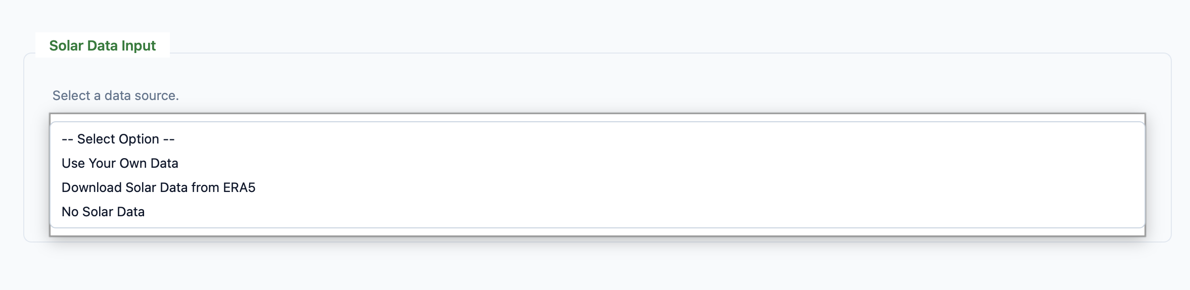
When using existing data, place solar_sites.csv and gen_all_sites.csv in the Solar directory and select the validation option. Column names and site names must follow the formats described in Data Requirements.
When downloading data, enter the desired start and end years. ProGRESS downloads ERA5 weather data for each location in solar_sites.csv and uses pvlib (https://pvlib-python.readthedocs.io/) to convert the weather data into solar generation profiles.
After solar generation data have been prepared, proceed to the clustering page.
ProGRESS uses k-means clustering to group days with similar solar-generation profiles. During the Monte Carlo simulation, representative days are sampled according to month-specific cluster probabilities.
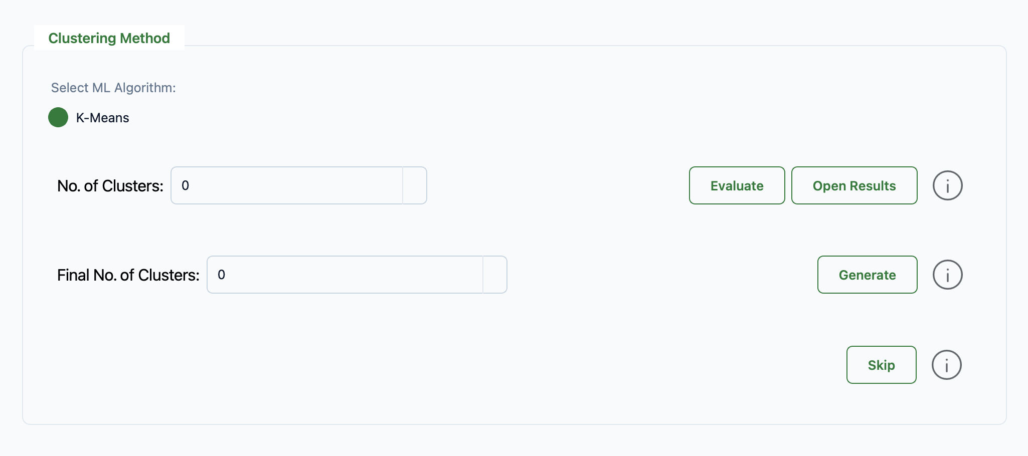
The clustering page provides two operations:
- Evaluate clusters: Evaluate a range of cluster counts using metrics such as the sum of squared errors and silhouette score.
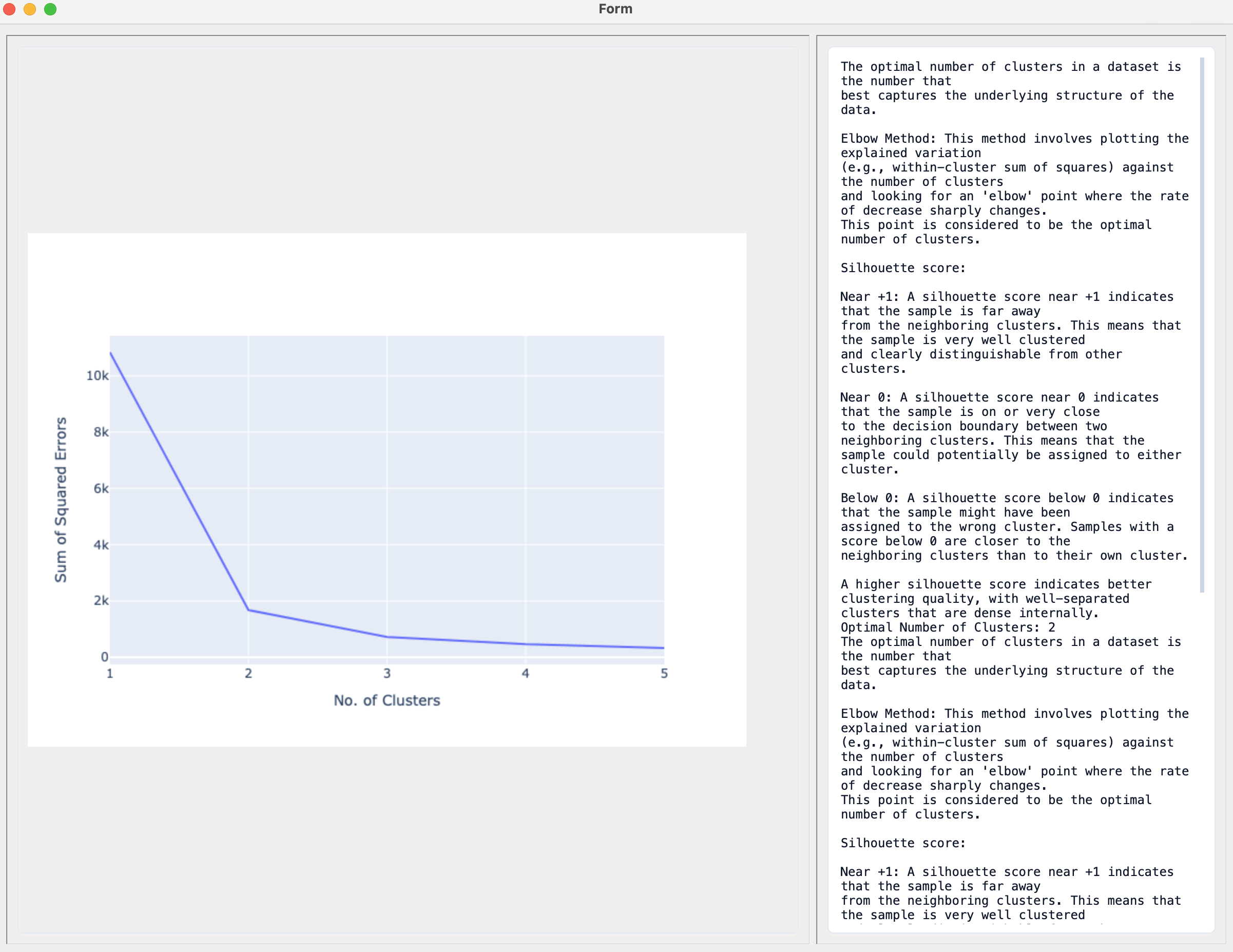
- Generate clusters: Select the final number of clusters and generate the cluster profiles and monthly probabilities used by the simulation.
The clustering process creates:
If valid cluster files have already been generated previously, the clustering process can be skipped.
If the system contains no solar generation, select No Solar Data.
On the Wind page, select one of the available data sources:
- Use Your Own Data
- Download Wind Data from ERA5
- No Wind Data
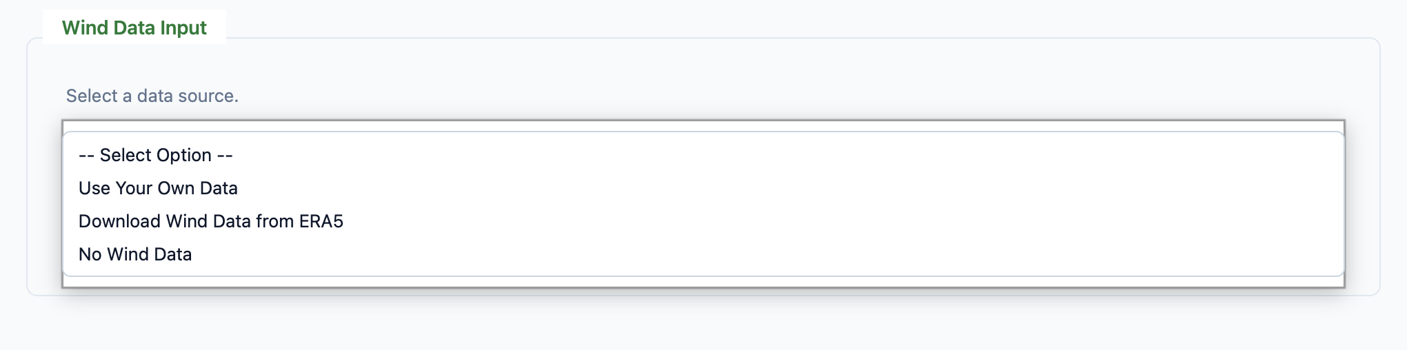
When using existing data, place wind_sites.csv, w_power_curves.csv, and windspeed_data.csv in the Wind directory and validate the files.
When downloading data, enter the desired start and end years. ProGRESS downloads ERA5 wind data for each location in wind_sites.csv and calculates the corresponding wind-speed time series.
Wind-speed data must be processed before running a simulation. Select Process Wind Data to generate the transition-rate matrices used by the stochastic wind model:
This processing step can be skipped if a valid t_rate.xlsx file already exists.
If the system contains no wind generation, select No Wind Data.
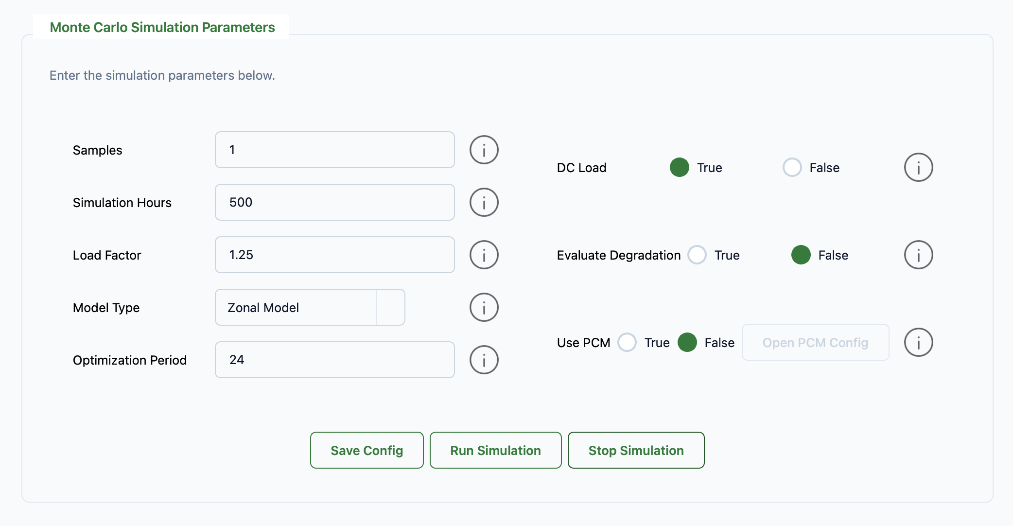
The Simulation page provides the following settings:
| Setting | Description |
|---|---|
| Samples | Number of Monte Carlo samples to run. |
| Simulation Hours | Number of simulated hours per sample. Use 8760 for a full non-leap year. |
| Load Factor | Multiplier applied to the base load at every bus. The default is 1. |
| Model Type | Network representation: Copper Sheet, Zonal, or Nodal. |
| Optimization Period | Use 1 for single-period reliability operation or a multiple of 24 for multi-period dispatch. |
| Data-Center Load | Enables randomly selected data-center load profiles. |
| Evaluate Degradation | Enables battery-capacity degradation during the simulation. |
| Degradation Interval | Number of hours between degradation evaluations. A value of at least 168 hours is recommended. |
| Detailed Thermal Model | Uses the PyBaMM thermal model instead of an assumed constant temperature of 25°C. |
| Use PCM | Enables co-simulation with the QuESt Production Cost Model. |
The available network models are:
- Copper Sheet: Ignores transmission constraints and provides the fastest generation-adequacy calculation.
- Zonal: Aggregates buses within each zone and represents power transfers between zones.
- Nodal: Retains the full bus and transmission network for the highest modeling fidelity.
Select Save Input to save the displayed settings to input.yaml.
When degradation is enabled, ProGRESS evaluates capacity fade using the battery chemistry specified in storage.csv. Supported chemistries are:
- LMO
- LFP
- NMC
- NCA
The detailed thermal model increases the simulation time substantially. Disable it to use a constant cell temperature of 25°C.
When data-center loads are enabled, ProGRESS randomly selects a profile from the following directory:
The selected profile is added to the matching system load columns for each Monte Carlo sample. For a zonal simulation, ProGRESS aggregates bus-level data-center profiles by zone.
When PCM is enabled, select PCM Configuration and provide:
- Path to the Python executable in the QuESt PCM environment
- Simulation start date
- Optimization solver
- MIP gap
- Pricing-problem option
- Storage ancillary-service participation option
PCM integration currently requires:
- The Nodal network model
- A 24-hour optimization period
- A separately installed QuESt PCM environment
*PCM and battery degradation cannot currently be enabled in the same simulation.
Select Run Simulation to save the current configuration and start the simulation.
Each run creates a timestamped directory in the Results folder.
Simulation messages and progress information are displayed in the log window.
Open the Results page after the simulation finishes. The results browser can display:
- CSV tables
- Excel workbooks
- PDF plots
- PNG images
- Text and JSON files
- HTML and Plotly results
Each serial simulation uses the following general output structure:
- progress/Results/
- YYYY-MM-DD_HH-MM-SS/
- indices.csv
- config.txt
- bus_outage_summary.txt
- convergence and outage plots
- Sample_1/
- ESS_SOC.csv
- solar_gen.csv
- wind_gen.csv
- outage records
- sample-level plots
- YYYY-MM-DD_HH-MM-SS/
The exact files depend on the selected model, number of samples, simulation length, variable generation, degradation settings, and PCM settings.
The calculated reliability indices include:
| Index | Description |
|---|---|
| LOLP | Loss-of-load probability |
| LOLH | Expected loss-of-load hours |
| LOLE | Loss-of-load expectation |
| LOLF | Loss-of-load frequency |
| EUE | Expected unserved energy |
| EPNS | Expected power not supplied |
| MDT | Mean outage duration |
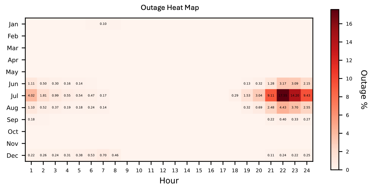
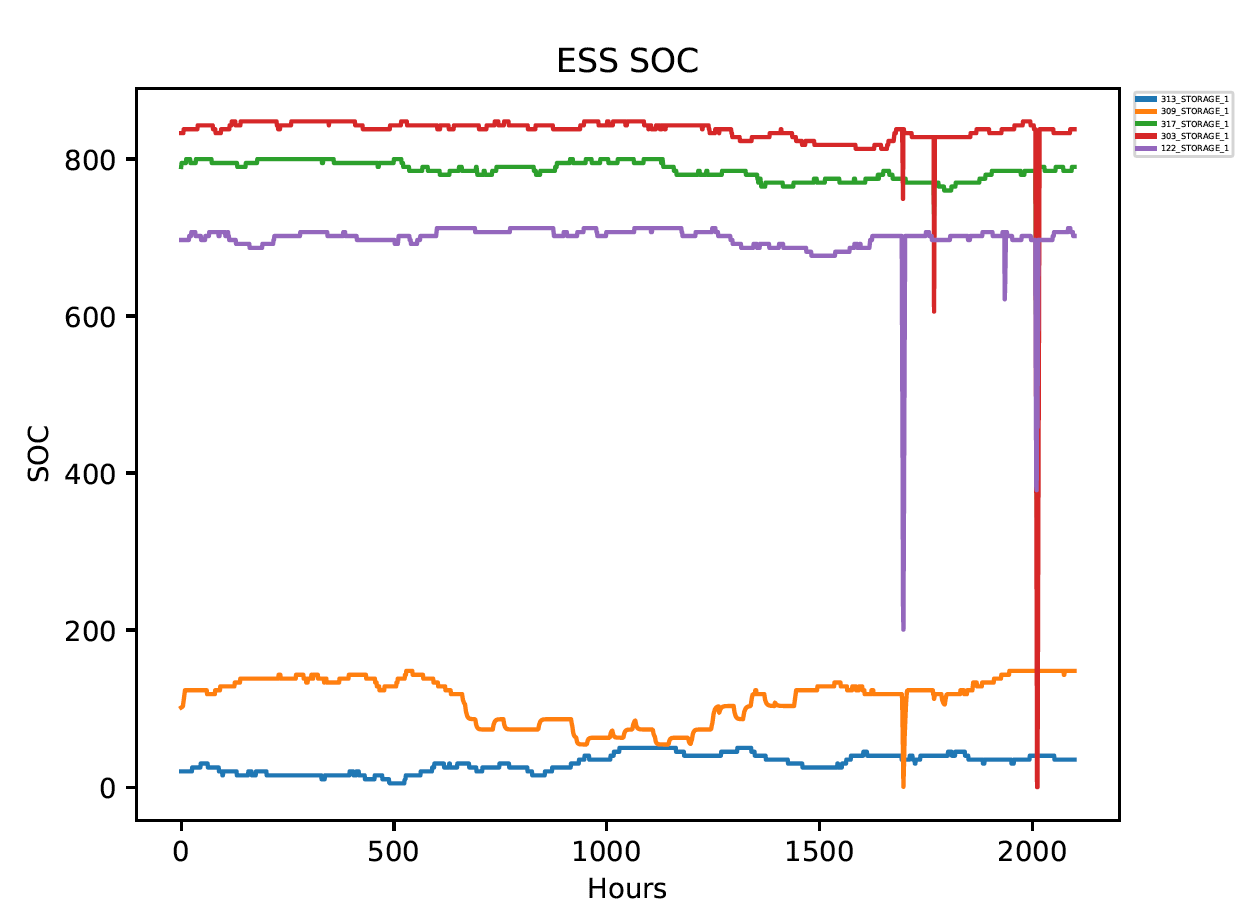
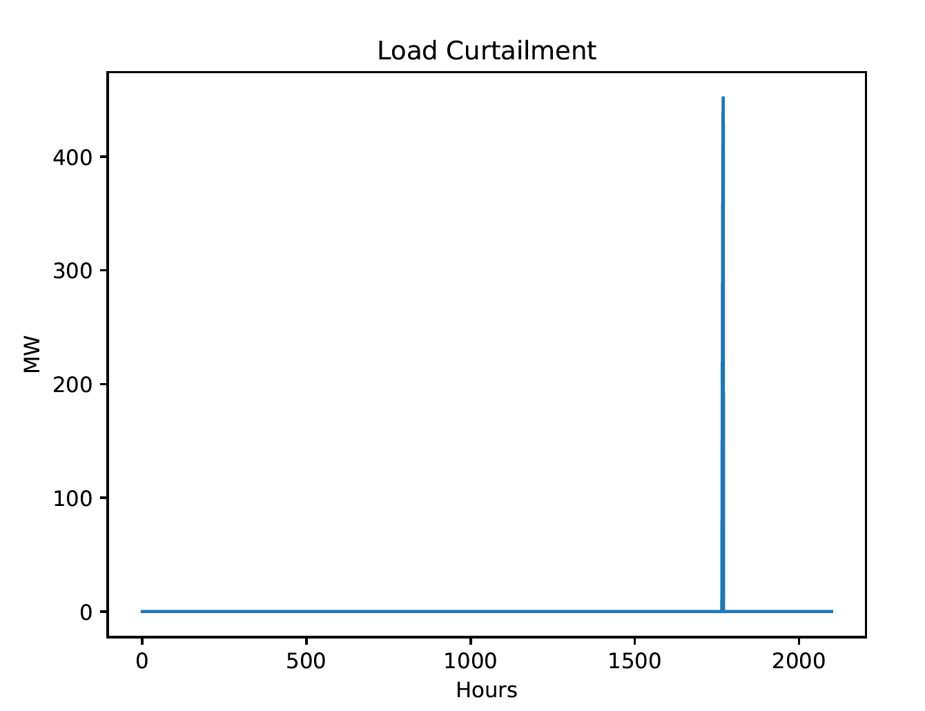
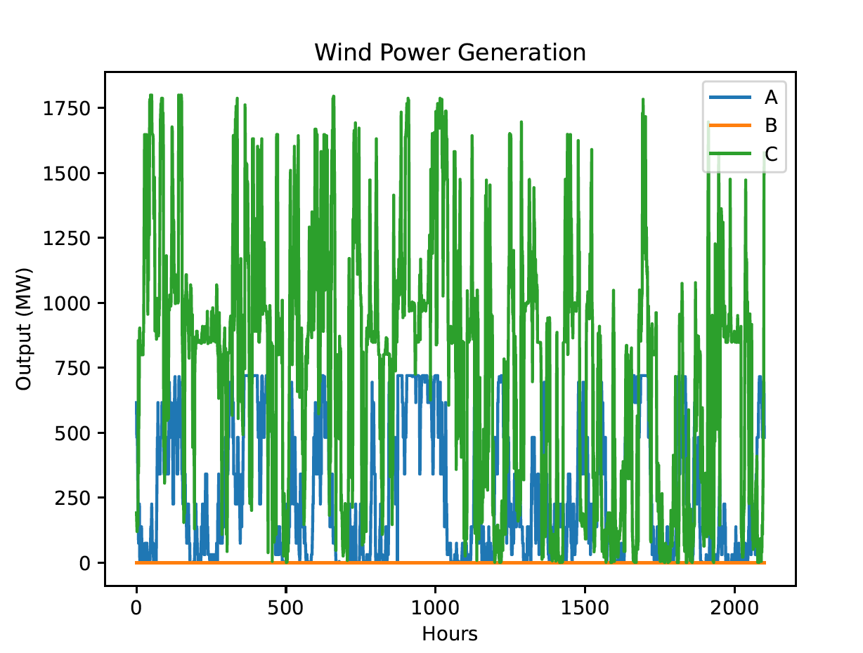
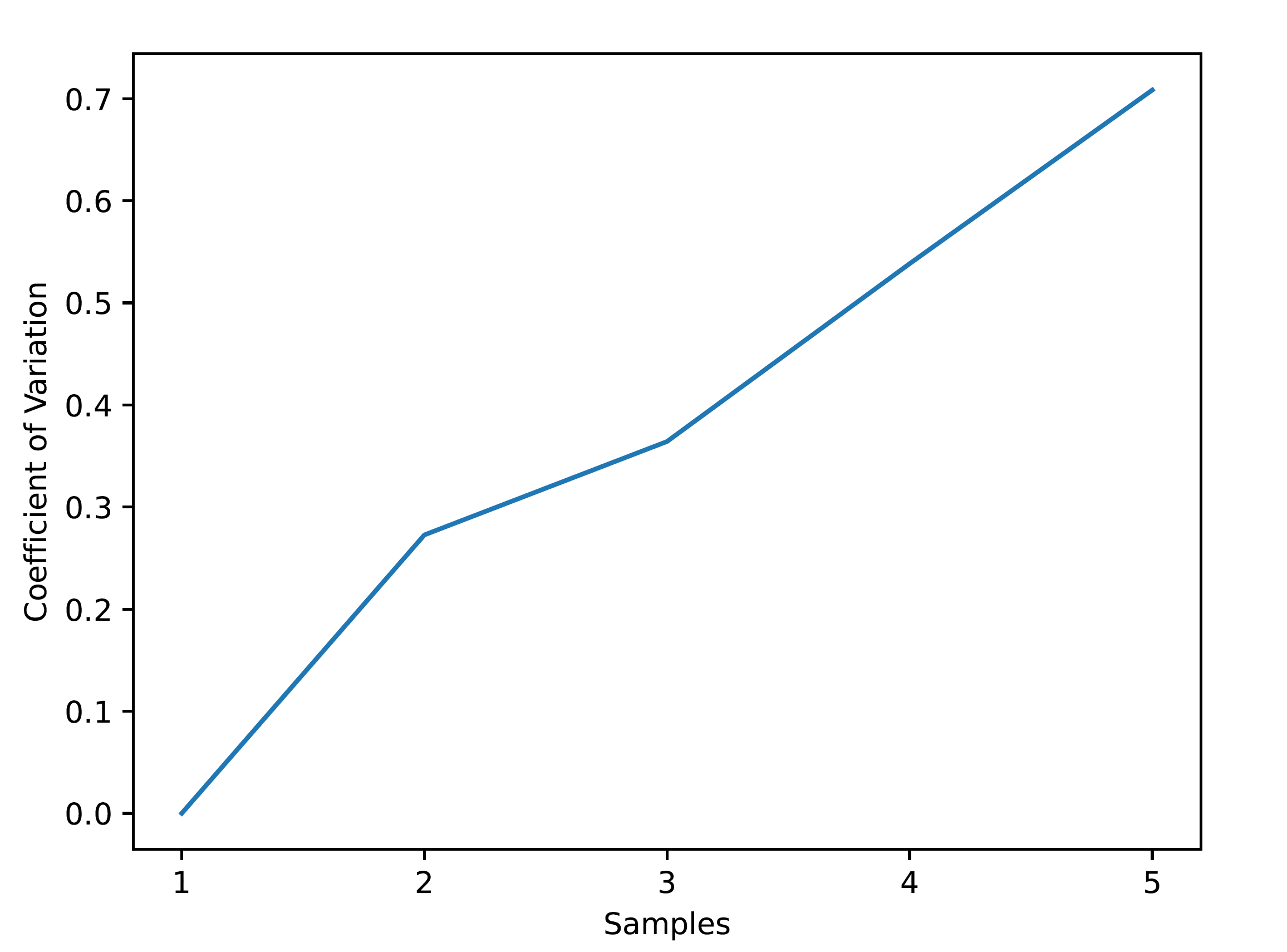
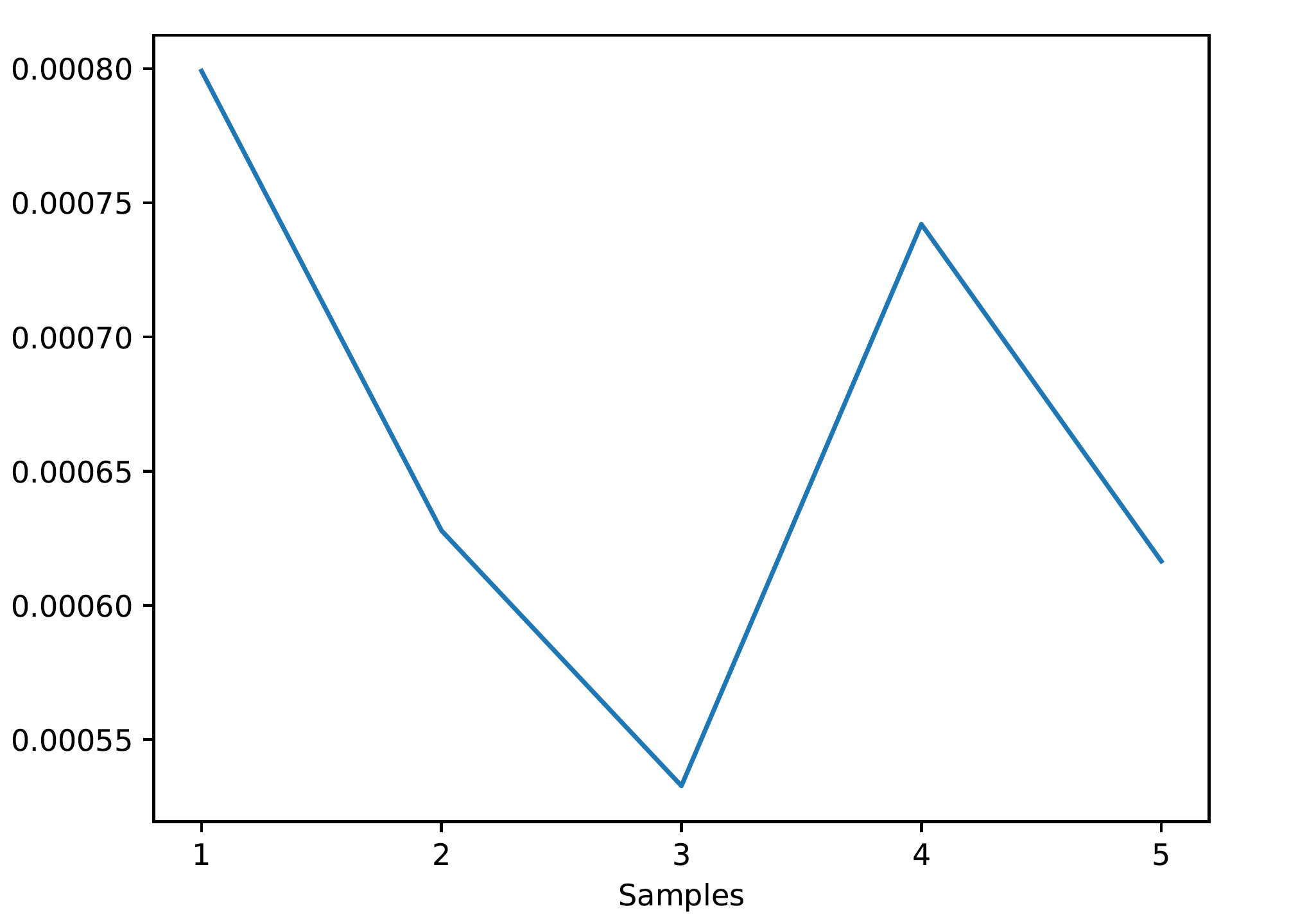
Outage heat maps are generated for full-year simulations of 8,760 hours. LOLP and coefficient-of-variation convergence plots are generated when multiple samples and nonzero loss-of-load events are available. Status of components such as generators, transmission lines, VERs, and ESS are recorded during the outage hours for in-depth analysis. Magnitude and duration of outages at all buses are also summarized for the simulation duration.
 |
 |
 |
 |
 |
 |
ProGRESS simulations can be prepared and executed without the GUI on a local computer or remote server.
Run all module commands from the repository root with the ProGRESS environment activated.
Edit the input.yaml to change configuration.
The primary configuration options are:
| Parameter | Description |
|---|---|
| data | Path to the root data directory. |
| samples | Number of Monte Carlo samples to run. |
| sim_hours | Number of simulated hours per sample. Use 8760 for a full non-leap year. |
| load_factor | Multiplier applied to the base load at every bus. |
| model | Network representation: Copper Sheet, Zonal, or Nodal. |
| optimization_period | Use 1 for single-period reliability operation or a multiple of 24 for multi-period dispatch. |
| download_s | Whether solar weather data should be downloaded. |
| year_start_s, year_end_s | ERA5 solar-data year range. |
| n_clusters | Number of solar clusters to generate. |
| download_w | Whether wind weather data should be downloaded. |
| year_start_w, year_end_w | ERA5 wind-data year range. |
| evaluate_degradation | Enables battery-capacity degradation during the simulation. |
| degradation_interval | Number of hours between degradation evaluations. A value of at least 168 hours is recommended. |
| detailed_thermal_model | Uses the PyBaMM thermal model instead of an assumed constant temperature of 25°C. |
| DC_load | Enables data-center load profiles. |
| use_pcm | Enables co-simulation with the QuESt Production Cost Model. |
PCM-specific options are stored under pcm_parameters.
If variable generation data must be downloaded or processed, run:
python -m progress.data_download_process
This workflow can:
- Download ERA5 meteorological data required for calculating VER generation.
- Convert solar weather data to solar generation
- Generate solar clusters and monthly probabilities
- Generate wind transition-rate matrices
This step can be skipped when all required processed VER files already exist.
Run the simulation using the default configuration:
python -m progress.example_simulation
A different configuration file can be supplied with --config:
python -m progress.example_simulation \
    --config /path/to/input.yaml
A custom results directory can be supplied with --out:
python -m progress.example_simulation \
    --config /path/to/input.yaml \
    --out /path/to/results
If --out is omitted, ProGRESS creates a timestamped directory under progress/Results.
ProGRESS includes an MPI-enabled simulation for running additional Monte Carlo samples across multiple processes. This workflow is intended for large systems, long simulations, or convergence studies requiring many samples.
An MPI runtime and the mpi4py Python package must be available on the computing system.
From the repository root, run:
mpiexec -n x python -m progress.example_simulation_mult_proc \
    --config progress/input.yaml \
    --out /path/to/results
Replace x with the desired number of MPI processes.
The samples setting is applied to each MPI process. Therefore, the total number of simulated samples is:
total samples = samples x MPI processes
Rank zero aggregates the reliability indices and generates the combined convergence and outage results.
The exact scheduler command and resource directives depend on the computing facility. For a Slurm system, place the MPI command in an appropriate batch script and submit it with:
sbatch your_job_script.bash
Consult the documentation for the target HPC system when selecting the number of nodes, tasks, memory, wall time, account, and partition.
Next: Additional Features — Degradation models, PCM integration, and multi-period optimization.