Home
The following details the steps involved in:
- Generating a Trinity de novo RNA-Seq assembly
- Evaluating the quality of the assembly
- Quantifying transcript expression levels
- Identifying differentially expressed (DE) transcripts
- Functionally annotating transcripts using Trinotate and predicting coding regions using TransDecoder
- Examining functional enrichments for DE transcripts using GOseq
- Interactively Exploring annotations and expression data via TrinotateWeb
All required software and data are provided pre-installed on the Amazon EC2 AMI. Be sure to have a running instance on at least an m4.large instance type, so we'll have adequate computational resources allocated in addition to reasonable response times over the network.
After launching and connecting to your running instance of the AMI, change your working directory to the base directory of these workshop materials:
% cd workshop_data/transcriptomics/KrumlovTrinityWorkshopJan2016/
For this course we will be using the data from this paper: Defining the transcriptomic landscape of Candida glabrata by RNA-Seq. Linde et al. Nucleic Acids Res. 2015 <http://www.ncbi.nlm.nih.gov/pubmed/?term=25586221 /> This work provides a detailed RNA-Seq-based analysis of the transcriptomic landscape of C. glabrata in nutrient-rich media (WT), as well as under nitrosative stress (GSNO), in addition to other conditions, but we'll restrict ourselves to just WT and GSNO conditions for demonstration purposes in this workshop.
There are paired-end FASTQ formatted Illlumina read files for each of the two conditions, with three biological replicates for each. All RNA-Seq data sets can be found in the data/ subdirectory:
% ls -1 data | grep fastq
.
GSNO_SRR1582646_1.fastq.gz
GSNO_SRR1582646_2.fastq.gz
GSNO_SRR1582647_1.fastq.gz
GSNO_SRR1582647_2.fastq.gz
GSNO_SRR1582648_1.fastq.gz
GSNO_SRR1582648_2.fastq.gz
wt_SRR1582649_1.fastq.gz
wt_SRR1582649_2.fastq.gz
wt_SRR1582650_1.fastq.gz
wt_SRR1582650_2.fastq.gz
wt_SRR1582651_1.fastq.gz
wt_SRR1582651_2.fastq.gz
Each biological replicate (eg. wt_SRR1582651) contains a pair of fastq files (eg. wt_SRR1582651_1.fastq.gz for the 'left' and wt_SRR1582651_2.fastq.gz for the 'right' read of the paired end sequences). Normally, each file would contain millions of reads, but in order to reduce running times as part of the workshop, each file provided here is restricted to only 10k RNA-Seq reads.
Below, we refer to '%' as the terminal command prompt, and we use environmental variables such as $TRINITY_HOME and $TRINOTATE_HOME as shortcuts to referring to their installation directories in the AMI image. To view the path to the installation directories, you can simply run:
% echo $TRINITY_HOME
Also, some commands can be fairly long to type in, an so they'll be more easily displayed in this document, we separate parts of the command with '' characters and put the rest of the command on the following line. Similarly in unix you can type '[return]' and you can continue to type in the rest of the command on the new line in the terminal.
For viewing text files, we'll use the unix utilities 'head' (look at the top few lines), 'cat' (print the entire contents of the file), and 'less' (interactively page through the file), and for viewing PDF formatted files, we'll use the 'xpdf' viewer utility.
To generate a reference assembly that we can later use for analyzing differential expression, we'll combine the read data sets for the different conditions together into a single target for Trinity assembly. We do this by providing Trinity with a list of all the left and right fastq files to the --left and --right parameters as comma-delimited like so:
   %   ${TRINITY_HOME}/Trinity --seqType fq  \
           --left data/wt_SRR1582649_1.fastq,data/wt_SRR1582651_1.fastq,data/wt_SRR1582650_1.fastq,data/GSNO_SRR1582648_1.fastq,data/GSNO_SRR1582646_1.fastq,data/GSNO_SRR1582647_1.fastq \
          --right data/wt_SRR1582649_2.fastq,data/wt_SRR1582651_2.fastq,data/wt_SRR1582650_2.fastq,data/GSNO_SRR1582648_2.fastq,data/GSNO_SRR1582646_2.fastq,data/GSNO_SRR1582647_2.fastq \
          --CPU 4 --max_memory 2G --min_contig_length 150
Note, if you see a message about not being able to identify the version of Java, please just ignore it.
Running Trinity on this data set may take 10 to 15 minutes. You'll see it progress through the various stages, starting with Jellyfish to generate the k-mer catalog, then followed by Inchworm, Chrysalis, and finally Butterfly. Running a typical Trinity job requires ~1 hour and ~1G RAM per ~1 million PE reads. You'd normally run it on a high-memory machine and let it churn for hours or days.
The assembled transcripts will be found at 'trinity_out_dir/Trinity.fasta'.
Just to look at the top few lines of the assembled transcript fasta file, you can run:
% head trinity_out_dir/Trinity.fasta
and you can see the Fasta-formatted Trinity output:
>TRINITY_DN506_c0_g1_i1 len=171 path=[149:0-170] [-1, 149, -2]
TGAGTATGGTTTTGCCGGTTTGGCTGTTGGTGCAGCTTTGAAGGGCCTAAAGCCAATTGT
TGAATTCATGTCATTCAACTTCTCCATGCAAGCCATTGACCATGTCGTTAACTCGGCAGC
AAAGACACATTATATGTCTGGTGGTACCCAAAAATGTCAAATCGTGTTCAG
>TRINITY_DN512_c0_g1_i1 len=168 path=[291:0-167] [-1, 291, -2]
ATATCAGCATTAGACAAAAGATTGTAAAGGATGGCATTAGGTGGTCGAAGTTTCAGGTCT
AAGAAACAGCAACTAGCATATGACAGGAGTTTTGCAGGCCGGTATCAGAAATTGCTGAGT
AAGAACCCATTCATATTCTTTGGACTCCCGTTTTGTGGAATGGTGGTG
>TRINITY_DN538_c0_g1_i1 len=310 path=[575:0-309] [-1, 575, -2]
GTTTTCCTCTGCGATCAAATCGTCAAACCTTAGACCTAGCTTGCGGTAACCAGAGTACTT
Note, the sequences you see will likely be different, as the order of sequences in the output is not deterministic.
Count the number of assembled transcripts
% grep '>' trinity_out_dir/Trinity.fasta | wc -l
How many were assembled?
Capture some basic statistics about the Trinity assembly:
% $TRINITY_HOME/util/TrinityStats.pl trinity_out_dir/Trinity.fasta
which should generate data like so. Note your numbers may vary slightly, as the assembly results are not deterministic.
################################
## Counts of transcripts, etc.
################################
Total trinity 'genes':	695
Total trinity transcripts:	695
Percent GC: 44.43

########################################
Stats based on ALL transcript contigs:
########################################

Contig N10: 656
Contig N20: 511
Contig N30: 420
Contig N40: 337
Contig N50: 284

Median contig length: 214
Average contig: 274.44
Total assembled bases: 190738


#####################################################
## Stats based on ONLY LONGEST ISOFORM per 'GENE':
#####################################################

Contig N10: 656
Contig N20: 511
Contig N30: 420
Contig N40: 337
Contig N50: 284

Median contig length: 214
Average contig: 274.44
Total assembled bases: 190738
To estimate the expression levels of the Trinity-reconstructed transcripts, we use the strategy supported by the RSEM software. We first align the original rna-seq reads back against the Trinity transcripts, then run RSEM to estimate the number of rna-seq fragments that map to each contig. Because the abundance of individual transcripts may significantly differ between samples, the reads from each sample (and each biological replicate) must be examined separately, obtaining sample-specific abundance values.
We include a script to faciliate running of RSEM on Trinity transcript assemblies. The script we execute below will run the Bowtie aligner to align reads to the Trinity transcripts, and RSEM will then evaluate those alignments to estimate expression values. Again, we need to run this separately for each sample and biological replicate (ie. each pair of fastq files).
Let's start with one of the GSNO treatment fastq pairs like so:
 %  $TRINITY_HOME/util/align_and_estimate_abundance.pl --seqType fq \
         --left data/GSNO_SRR1582648_1.fastq \
         --right data/GSNO_SRR1582648_2.fastq  \
         --transcripts trinity_out_dir/Trinity.fasta  \
         --output_prefix GSNO_SRR1582648 \
         --est_method RSEM  --aln_method bowtie \
         --trinity_mode --prep_reference --coordsort_bam \
         --output_dir GSNO_SRR1582648.RSEM
The outputs generated from running the command above will exist in the GSNO_SRR1582648.RSEM/ directory, as we indicate with the --output_dir parameter above.
The primary output generated by RSEM is the file containing the expression values for each of the transcripts. Examine this file like so:
% head GSNO_SRR1582648.RSEM/GSNO_SRR1582648.isoforms.results
and you should see the top of a tab-delimited file:
transcript_id	gene_id	length	effective_length	expected_count	TPM	FPKM	IsoPct
TRINITY_DN0_c0_g1_i1	TRINITY_DN0_c0_g1	1068	938.62	0.00	0.00	0.00	0.00
TRINITY_DN100_c0_g1_i1	TRINITY_DN100_c0_g1	329	199.75	4.00	1247.60	6022.67	100.00
TRINITY_DN101_c0_g1_i1	TRINITY_DN101_c0_g1	221	92.28	0.00	0.00	0.00	0.00
TRINITY_DN102_c0_g1_i1	TRINITY_DN102_c0_g1	214	85.39	0.00	0.00	0.00	0.00
TRINITY_DN103_c0_g1_i1	TRINITY_DN103_c0_g1	342	212.72	1.00	292.87	1413.82	100.00
TRINITY_DN104_c0_g1_i1	TRINITY_DN104_c0_g1	185	57.37	0.00	0.00	0.00	0.00
TRINITY_DN105_c0_g1_i1	TRINITY_DN105_c0_g1	417	287.65	44.00	9529.91	46004.65	100.00
TRINITY_DN106_c0_g1_i1	TRINITY_DN106_c0_g1	189	61.16	0.00	0.00	0.00	0.00
TRINITY_DN107_c0_g1_i1	TRINITY_DN107_c0_g1	333	203.74	0.00	0.00	0.00	0.00
The key columns in the above RSEM output are the transcript identifier, the 'expected_count' corresponding to the number of RNA-Seq fragments predicted to be derived from that transcript, and the 'TPM' or 'FPKM' columns, which provide normalized expression values for the expression of that transcript in the sample. TPM is generally the favored metric, as all TPM values should sum to 1 million, and TPM nicely reflects the relative molar concentration of that transcript in the sample.
Running this on all the samples can be montonous, and with many more samples, advanced users would generally write a short script to fully automate this process. We won't be scripting here, but instead just directly execute abundance estimation just as we did above but on the other five pairs of fastq files. We'll examine the outputs of each in turn, as a sanity check and also just for fun.
Process fastq pair 2:
 % $TRINITY_HOME/util/align_and_estimate_abundance.pl --seqType fq  \
         --left data/GSNO_SRR1582646_1.fastq \
         --right data/GSNO_SRR1582646_2.fastq \
         --transcripts trinity_out_dir/Trinity.fasta \
         --output_prefix GSNO_SRR1582646 \
         --est_method RSEM  --aln_method bowtie \
         --trinity_mode --prep_reference --coordsort_bam  \
         --output_dir GSNO_SRR1582646.RSEM

  % head GSNO_SRR1582646.RSEM/GSNO_SRR1582646.isoforms.results
Process fastq pair 3:
 % $TRINITY_HOME/util/align_and_estimate_abundance.pl --seqType fq \
    --left data/GSNO_SRR1582647_1.fastq \
    --right data/GSNO_SRR1582647_2.fastq \
    --transcripts trinity_out_dir/Trinity.fasta  \
    --output_prefix GSNO_SRR1582647 \
    --est_method RSEM --aln_method bowtie --trinity_mode \
    --prep_reference --coordsort_bam  \
    --output_dir GSNO_SRR1582647.RSEM

 % head GSNO_SRR1582647.RSEM/GSNO_SRR1582647.isoforms.results
Now we're done with processing the GSNO-treated biological replicates, and we'll proceed to now run abundance estimations for the WT samples.
Process fastq pair 4:
 % $TRINITY_HOME/util/align_and_estimate_abundance.pl --seqType fq \
     --left data/wt_SRR1582649_1.fastq \
     --right data/wt_SRR1582649_2.fastq \
     --transcripts trinity_out_dir/Trinity.fasta \
     --output_prefix wt_SRR1582649 \
     --est_method RSEM  --aln_method bowtie --trinity_mode \
     --prep_reference --coordsort_bam  \
     --output_dir wt_SRR1582649.RSEM


 % head wt_SRR1582649.RSEM/wt_SRR1582649.isoforms.results
Process fastq pair 5:
% $TRINITY_HOME/util/align_and_estimate_abundance.pl --seqType fq \
     --left data/wt_SRR1582651_1.fastq \
     --right data/wt_SRR1582651_2.fastq  \
     --transcripts trinity_out_dir/Trinity.fasta \
     --output_prefix wt_SRR1582651 \
     --est_method RSEM  --aln_method bowtie --trinity_mode \
     --prep_reference --coordsort_bam  \
     --output_dir wt_SRR1582651.RSEM

% head wt_SRR1582651.RSEM/wt_SRR1582651.isoforms.results
Process fastq pair 6 (last one!!):
% $TRINITY_HOME/util/align_and_estimate_abundance.pl --seqType fq \
     --left data/wt_SRR1582650_1.fastq \
     --right data/wt_SRR1582650_2.fastq \
     --transcripts trinity_out_dir/Trinity.fasta \
     --output_prefix wt_SRR1582650\
     --est_method RSEM  --aln_method bowtie --trinity_mode \
     --prep_reference --coordsort_bam  \
     --output_dir wt_SRR1582650.RSEM

% head wt_SRR1582650.RSEM/wt_SRR1582650.isoforms.results
Now, given the expression estimates for each of the transcripts in each of the samples, we're going to pull together all values into matrices containing transcript IDs in the rows, and sample names in the columns. We'll make two matrices, one containing the estimated counts, and another containing the TPM expression values that are cross-sample normalized using the TMM method. This is all done for you by the following script in Trinity, indicating the method we used for expresssion estimation and providing the list of individual sample abundance estimate files:
% $TRINITY_HOME/util/abundance_estimates_to_matrix.pl --est_method RSEM \
      --out_prefix Trinity_trans \
      GSNO_SRR1582648.RSEM/GSNO_SRR1582648.isoforms.results \
      GSNO_SRR1582646.RSEM/GSNO_SRR1582646.isoforms.results \
      GSNO_SRR1582647.RSEM/GSNO_SRR1582647.isoforms.results \
      wt_SRR1582649.RSEM/wt_SRR1582649.isoforms.results \
      wt_SRR1582651.RSEM/wt_SRR1582651.isoforms.results \
      wt_SRR1582650.RSEM/wt_SRR1582650.isoforms.results
You should find a matrix file called 'Trinity_trans.counts.matrix', which contains the counts of RNA-Seq fragments mapped to each transcript. Examine the first few lines of the counts matrix:
% head -n20 Trinity_trans.counts.matrix
.
    GSNO_SRR1582648	GSNO_SRR1582646	GSNO_SRR1582647	wt_SRR1582649	wt_SRR1582651	wt_SRR1582650
TRINITY_DN541_c0_g1_i1	0.00	0.00	0.00	1.00	1.00	1.00
TRINITY_DN593_c0_g1_i1	0.00	0.00	0.00	0.00	0.00	0.00
TRINITY_DN496_c0_g1_i1	1.00	0.00	0.00	2.00	1.00	6.00
TRINITY_DN658_c0_g1_i1	0.00	0.00	0.00	1.00	1.00	1.00
TRINITY_DN416_c0_g1_i1	2.00	0.00	3.00	1.00	6.00	2.00
TRINITY_DN301_c0_g1_i1	0.00	2.00	3.00	1.00	0.00	0.00
TRINITY_DN413_c0_g1_i1	2.00	2.00	2.00	0.00	0.00	0.00
TRINITY_DN218_c0_g1_i1	0.00	1.00	1.00	7.00	4.00	1.00
TRINITY_DN387_c0_g1_i1	0.00	0.00	2.00	4.00	2.00	4.00
TRINITY_DN220_c0_g1_i1	14.00	32.00	26.00	1.00	3.00	2.00
TRINITY_DN506_c0_g1_i1	0.00	0.00	0.00	1.00	0.00	3.00
TRINITY_DN94_c0_g1_i1	0.00	0.00	0.00	1.00	3.00	4.00
TRINITY_DN671_c0_g1_i1	0.00	1.00	1.00	1.00	0.00	1.00
TRINITY_DN69_c0_g1_i1	0.00	1.00	0.00	2.00	0.00	2.00
TRINITY_DN427_c0_g1_i1	1.00	1.00	0.00	3.00	2.00	2.00
TRINITY_DN311_c0_g1_i1	0.00	2.00	3.00	3.00	1.00	4.00
TRINITY_DN75_c0_g1_i1	0.00	0.00	1.00	0.00	0.00	0.00
TRINITY_DN670_c0_g1_i1	0.00	0.00	0.00	1.00	1.00	2.00
TRINITY_DN174_c0_g1_i1	0.00	2.00	0.00	5.00	5.00	4.00
And now take a look at the first few lines of the normalized expression matrix:
% head -n20 Trinity_trans.TMM.EXPR.matrix
.
   	GSNO_SRR1582648	GSNO_SRR1582646	GSNO_SRR1582647	wt_SRR1582649	wt_SRR1582651	wt_SRR1582650
TRINITY_DN541_c0_g1_i1	0.000	0.000	0.000	1654.976	2535.416	1673.349
TRINITY_DN593_c0_g1_i1	0.000	0.000	0.000	0.000	0.000	0.000
TRINITY_DN496_c0_g1_i1	580.099	0.000	0.000	1119.697	692.351	3545.149
TRINITY_DN658_c0_g1_i1	0.000	0.000	0.000	667.237	854.024	700.959
TRINITY_DN416_c0_g1_i1	833.626	0.000	1105.023	403.956	2826.946	858.922
TRINITY_DN301_c0_g1_i1	0.000	1618.849	2264.871	800.529	0.000	0.000
TRINITY_DN413_c0_g1_i1	938.144	878.406	831.524	0.000	0.000	0.000
TRINITY_DN218_c0_g1_i1	0.000	352.406	335.147	2581.019	1694.620	392.566
TRINITY_DN387_c0_g1_i1	0.000	0.000	630.894	1390.755	791.766	1481.920
TRINITY_DN220_c0_g1_i1	1579.873	3248.668	2549.425	110.156	336.120	236.830
TRINITY_DN506_c0_g1_i1	0.000	0.000	0.000	1200.525	0.000	3695.785
TRINITY_DN94_c0_g1_i1	0.000	0.000	0.000	490.353	1774.642	2076.616
TRINITY_DN671_c0_g1_i1	0.000	1900.917	1719.015	1745.562	0.000	1760.231
TRINITY_DN69_c0_g1_i1	0.000	835.148	0.000	1647.701	0.000	1718.149
TRINITY_DN427_c0_g1_i1	1532.057	1563.879	0.000	4385.116	4365.486	2973.535
TRINITY_DN311_c0_g1_i1	0.000	1295.009	1822.198	1954.968	830.244	2740.275
TRINITY_DN75_c0_g1_i1	0.000	0.000	1821.697	0.000	0.000	0.000
TRINITY_DN670_c0_g1_i1	0.000	0.000	0.000	1363.976	2008.630	2783.536
TRINITY_DN174_c0_g1_i1	0.000	2698.139	0.000	6387.351	9282.501	5228.969
% $TRINITY_HOME/util/misc/contig_ExN50_statistic.pl Trinity_trans.TMM.EXPR.matrix trinity_out_dir/Trinity.fasta > ExN50.stats
View the contents of the above output file:
% cat ExN50.stats
.
#E	min_expr	E-N50	num_transcripts
E1	28800.870	247	1
E3	28800.870	328	2
E4	18270.379	247	3
E5	18270.379	258	4
E6	17095.704	258	5
...
E24	5275.906	416	40
E25	5275.906	417	42
E26	5275.906	417	45
E27	5275.906	420	48
E28	5275.906	423	51
...
E61	1905.138	420	212
E62	1905.138	420	219
E63	1905.138	420	226
E64	1905.138	420	233
E65	1905.138	420	241
E66	1905.138	417	249
...
E91	947.708	320	511
E92	947.708	315	525
E93	947.708	313	540
E94	947.708	313	555
E95	947.708	309	571
E96	883.415	308	588
E97	806.468	305	607
E98	806.468	302	627
E99	607.700	297	650
E100	0.021	285	689
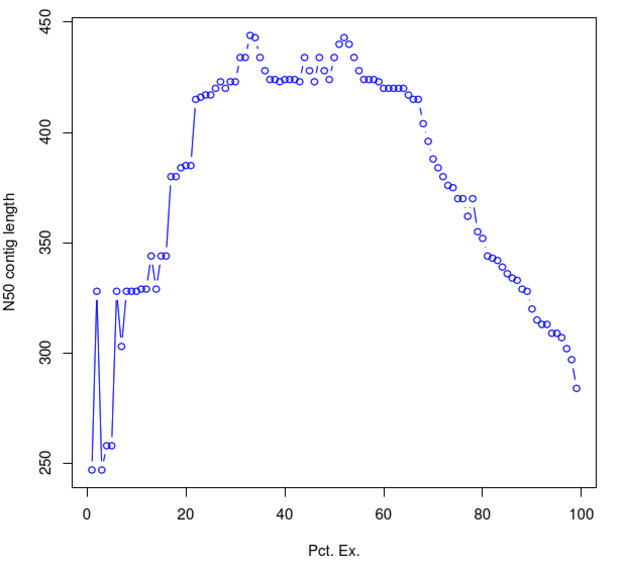
Plot the ExN50 statistics:
% $TRINITY_HOME/util/misc/plot_ExN50_statistic.Rscript ExN50.stats

% xpdf ExN50.stats.plot.pdf
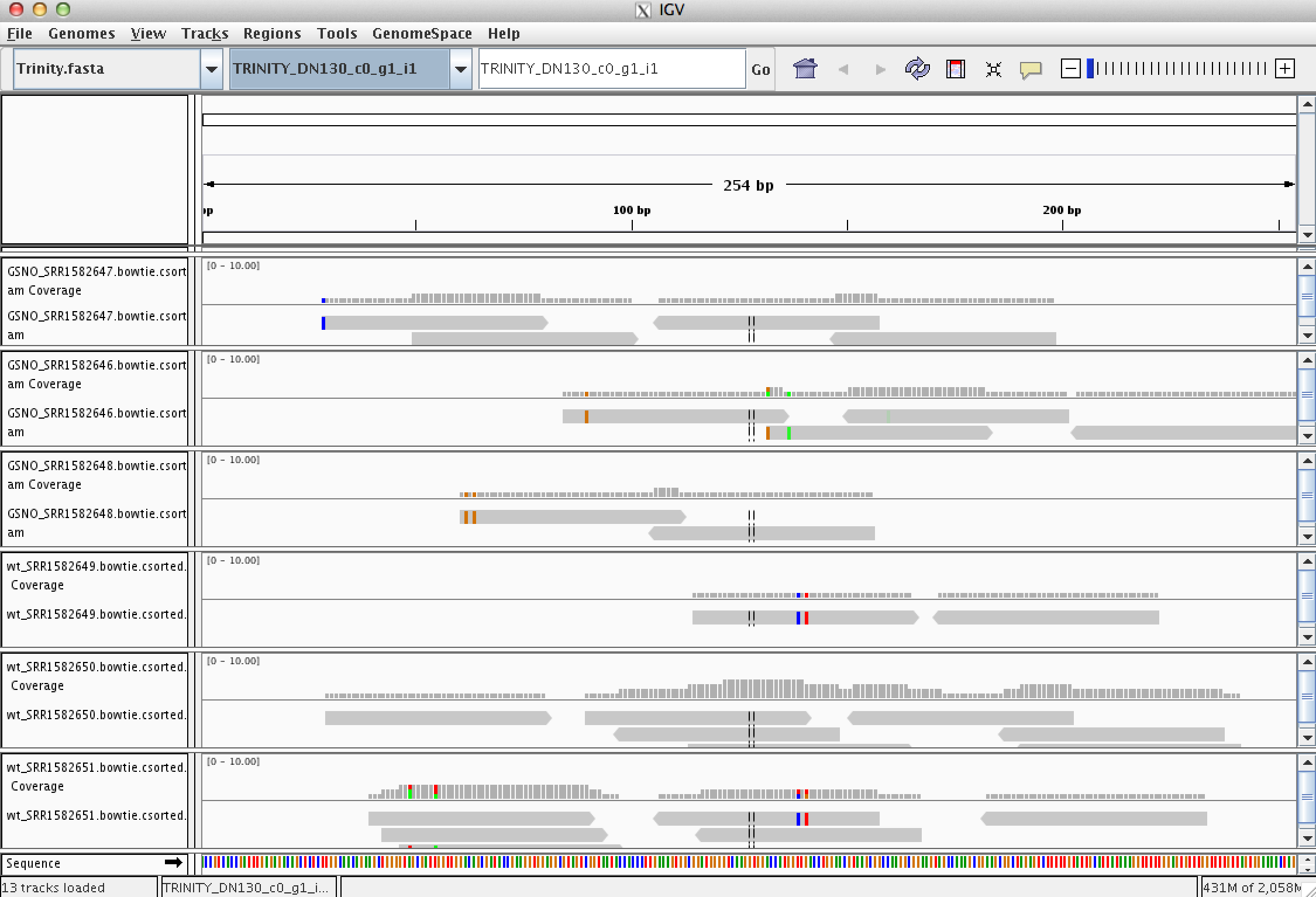
% igv.sh -g trinity_out_dir/Trinity.fasta \
    GSNO_SRR1582648.RSEM/GSNO_SRR1582648.bowtie.csorted.bam,GSNO_SRR1582646.RSEM/GSNO_SRR1582646.bowtie.csorted.bam,GSNO_SRR1582647.RSEM/GSNO_SRR1582647.bowtie.csorted.bam,wt_SRR1582651.RSEM/wt_SRR1582651.bowtie.csorted.bam,wt_SRR1582649.RSEM/wt_SRR1582649.bowtie.csorted.bam,wt_SRR1582650.RSEM/wt_SRR1582650.bowtie.csorted.bam
(description of DE analysis, need samples file)
% cat samples.txt

GSNO	GSNO_SRR1582648
GSNO	GSNO_SRR1582647
GSNO	GSNO_SRR1582646
WT	wt_SRR1582651
WT	wt_SRR1582649
WT	wt_SRR1582650
To detect differentially expressed transcripts, run the Bioconductor package edgeR using our counts matrix:
%  $TRINITY_HOME/Analysis/DifferentialExpression/run_DE_analysis.pl \
      --matrix Trinity_trans.counts.matrix \
      --samples_file samples.txt \
      --method edgeR \
      --output edgeR
Examine the contents of the edgeR/ directory.
% ls -ltr edgeR/
.
-rw-rw-r-- 1 genomics genomics  1051 Jan  9 16:48 Trinity_trans.counts.matrix.GSNO_vs_WT.GSNO.vs.WT.EdgeR.Rscript
-rw-rw-r-- 1 genomics genomics 60902 Jan  9 16:48 Trinity_trans.counts.matrix.GSNO_vs_WT.edgeR.DE_results
-rw-rw-r-- 1 genomics genomics 18537 Jan  9 16:48 Trinity_trans.counts.matrix.GSNO_vs_WT.edgeR.DE_results.MA_n_Volcano.pdf
The files '*.DE_results' contain the output from running EdgeR to identify differentially expressed transcripts in each of the pairwise sample comparisons. Examine the format of one of the files, such as the results from comparing Sp_log to Sp_plat:
% head edgeR/Trinity_trans.counts.matrix.GSNO_vs_WT.edgeR.DE_results
.
logFC	logCPM	PValue	FDR
TRINITY_DN437_c0_g1_i1	8.98959066402695	13.1228060448362	8.32165055033775e-54	5.54221926652494e-51
TRINITY_DN469_c0_g1_i1	4.89839016049723	13.2154341051504	7.57411107973887e-53	2.52217898955304e-50
TRINITY_DN46_c0_g1_i1	2.69777851490106	14.1332252828559	5.23937214153746e-52	1.16314061542132e-49
TRINITY_DN131_c0_g1_i1	5.96230500956404	13.4919132973162	5.11512415417842e-51	8.51668171670708e-49
TRINITY_DN278_c0_g1_i1	5.67480055313841	12.8660937412604	1.54064866426519e-44	2.05214402080123e-42
TRINITY_DN263_c0_g1_i1	8.97722926993194	13.108274725098	3.6100707178792e-44	4.00717849684591e-42
TRINITY_DN356_c0_g1_i1	2.71537635410452	14.0482419858984	8.00431159168039e-41	7.61553074294163e-39
TRINITY_DN0_c0_g1_i1	6.96733684710045	12.875060733337	3.67004658844109e-36	3.05531378487721e-34
TRINITY_DN59_c0_g1_i1	-3.57509574692799	13.1852604213653	3.74452542871713e-30	2.77094881725068e-28
These data include the log fold change (logFC), log counts per million (logCPM), P- value from an exact test, and false discovery rate (FDR).
The EdgeR analysis above generated both MA and Volcano plots based on these data. Examine any of these like so:
% xpdf edgeR/Trinity_trans.counts.matrix.GSNO_vs_WT.edgeR.DE_results.MA_n_Volcano.pdf
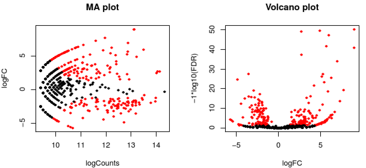
Exit the chart viewer to continue.
Trinity facilitates analysis of these data, including scripts for extracting transcripts that are above some statistical significance (FDR threshold) and fold-change in expression, and generating figures such as heatmaps and other useful plots, as described below.
Now let's perform the following operations from within the edgeR/ directory. Enter the edgeR/ dir like so:
% cd edgeR/
Extract those differentially expressed (DE) transcripts that are at least 4-fold differentially expressed at a significance of <= 0.001 in any of the pairwise sample comparisons:
% $TRINITY_HOME/Analysis/DifferentialExpression/analyze_diff_expr.pl \
      --matrix ../Trinity_trans.TMM.EXPR.matrix \
      --samples ../samples.txt \
      -P 1e-3 -C 2
The above generates several output files with a prefix diffExpr.P1e-3_C2', indicating the parameters chosen for filtering, where P (FDR actually) is set to 0.001, and fold change (C) is set to 2^(2) or 4-fold. (These are default parameters for the above script. See script usage before applying to your data).
Included among these files are: ‘diffExpr.P1e-3_C2.matrix’ : the subset of the FPKM matrix corresponding to the DE transcripts identified at this threshold. The number of DE transcripts identified at the specified thresholds can be obtained by examining the number of lines in this file.
% wc -l diffExpr.P1e-3_C2.matrix
.
116 diffExpr.P1e-3_C2.matrix
Note, the number of lines in this file includes the top line with column names, so there are actually 56 DE transcripts at this 4-fold and 1e-3 FDR threshold cutoff.
Also included among these files is a heatmap 'diffExpr.P1e-3_C2.matrix.log2.centered.genes_vs_samples_heatmap.pdf' as shown below, with transcripts clustered along the vertical axis and samples clustered along the horizontal axis.
% xpdf diffExpr.P1e-3_C2.matrix.log2.centered.genes_vs_samples_heatmap.pdf
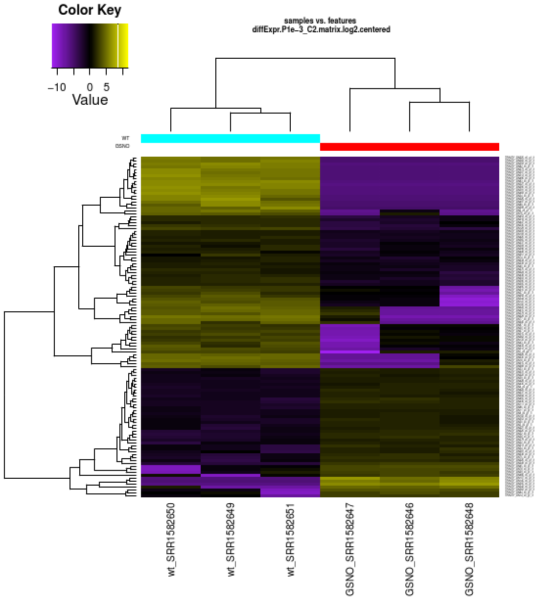
Exit the PDF viewer to continue.
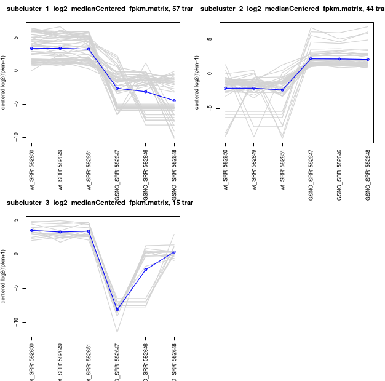
Extract clusters of transcripts with similar expression profiles by cutting the transcript cluster dendrogram at a given percent of its height (ex. 60%), like so:
% $TRINITY_HOME/Analysis/DifferentialExpression/define_clusters_by_cutting_tree.pl \
       --Ptree 60 -R diffExpr.P1e-3_C2.matrix.RData
This creates a directory containing the individual transcript clusters, including a pdf file that summarizes expression values for each cluster according to individual charts:
% xpdf diffExpr.P1e-3_C2.matrix.RData.clusters_fixed_P_60/my_cluster_plots.pdf
% cd ../

% mkdir Trinotate

% cd Trinotate

% ln -s ../trinity_out_dir/Trinity.fasta
% $TRANSDECODER_HOME/TransDecoder.LongOrfs -t Trinity.fasta

% $TRANSDECODER_HOME/TransDecoder.Predict -t Trinity.fasta
% blastx -db ../data/mini_sprot.pep -query Trinity.fasta -num_threads 2 -max_target_seqs 1 -outfmt 6 -evalue 1e-5 > swissprot.blastx.outfmt6


% blastp -query Trinity.fasta.transdecoder.pep -db ../data/mini_sprot.pep -num_threads 2 -max_target_seqs 1 -outfmt 6 -evalue 1e-5 > swissprot.blastp.outfmt6


% hmmscan --cpu 2 --domtblout TrinotatePFAM.out /home/genomics/workshop_data/transcriptomics/trinnotate_databases/Pfam-A.hmm Trinity.fasta.transdecoder.pep
Signal peptide prediction:
% signalp -f short -n signalp.out Trinity.fasta.transdecoder.pep
Transmembrane domain predictions
% tmhmm --short < Trinity.fasta.transdecoder.pep > tmhmm.out
%  ln -s ../Trinotate.sqlite

%  $TRINOTATE_HOME/Trinotate Trinotate.sqlite init --gene_trans_map ../trinity_out_dir/Trinity.fasta.gene_trans_map --transcript_fasta Trinity.fasta --transdecoder_pep Trinity.fasta.transdecoder.pep

%  $TRINOTATE_HOME/Trinotate Trinotate.sqlite LOAD_swissprot_blastx swissprot.blastx.outfmt6

%  $TRINOTATE_HOME/Trinotate Trinotate.sqlite LOAD_swissprot_blastp swissprot.blastp.outfmt6

%  $TRINOTATE_HOME/Trinotate Trinotate.sqlite LOAD_pfam TrinotatePFAM.out

%  $TRINOTATE_HOME/Trinotate Trinotate.sqlite LOAD_tmhmm tmhmm.out

%  $TRINOTATE_HOME/Trinotate Trinotate.sqlite LOAD_signalp signalp.out
% $TRINOTATE_HOME/Trinotate Trinotate.sqlite report > Trinotate.xls
View the report
% less Trinotate.xls
% $TRINOTATE_HOME/util/extract_GO_assignments_from_Trinotate_xls.pl --Trinotate_xls Trinotate.xls -T -I > Trinotate.xls.gene_ontology
If you see warning messages 'cannot parse parent info', simply ignore them.
%  $TRINOTATE_HOME/util/annotation_importer/import_transcript_names.pl Trinotate.sqlite Trinotate.xls

% cd ../edgeR

% $TRINITY_HOME/util/misc/fasta_seq_length.pl ../trinity_out_dir/Trinity.fasta > Trinity.seqLengths

%  $TRINITY_HOME/Analysis/DifferentialExpression/run_GOseq.pl --genes_single_factor Trinity_trans.counts.matrix.GSNO_vs_WT.edgeR.DE_results.P1e-3_C2.GSNO-UP.subset --GO_assignments ../Trinotate/Trinotate.xls.gene_ontology --lengths Trinity.seqLengths

%  $TRINITY_HOME/Analysis/DifferentialExpression/run_GOseq.pl --genes_single_factor Trinity_trans.counts.matrix.GSNO_vs_WT.edgeR.DE_results.P1e-3_C2.WT-UP.subset --GO_assignments ../Trinotate/Trinotate.xls.gene_ontology --lengths Trinity.seqLengths
% cd ../Trinotate

%  $TRINOTATE_HOME/util/transcript_expression/import_expression_and_DE_results.pl --sqlite Trinotate.sqlite --transcript_mode --samples_file ../samples.txt --count_matrix ../Trinity_trans.counts.matrix --fpkm_matrix ../Trinity_trans.TMM.EXPR.matrix

%  $TRINOTATE_HOME/util/transcript_expression/import_expression_and_DE_results.pl --sqlite Trinotate.sqlite --transcript_mode --samples_file ../samples.txt --DE_dir ../edgeR

%  $TRINOTATE_HOME/util/transcript_expression/import_transcript_clusters.pl --sqlite Trinotate.sqlite --group_name DE_all_vs_all --analysis_name diffExpr.P1e-3_C2.matrix.RData.clusters_fixed_P_60 ../edgeR/diffExpr.P1e-3_C2.matrix.RData.clusters_fixed_P_60/*matrix
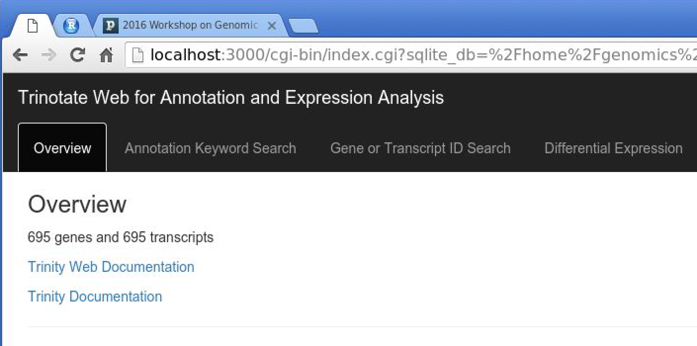
% $TRINOTATE_HOME/run_TrinotateWebserver.pl 3000